
By: Yusuf M. Khaled & Stephen Shiwei Wang
Edited By: Sayidcali Ahmed
Introduction
States across the United States have vastly different geological and geographical landscapes, and these differences support thousands of species. State biodiversity conservation needs vary substantially across the United States, reflecting differences in species richness, risk concentration, land area, and land-use pressure.1 Yet the observed distribution of conservation funding may not align closely with these measurable indicators of ecological burden. This raises a central policy question: whether current funding levels correspond to ecological needs or are systematically misaligned across states.
With a dataset of state-level biodiversity, land-cover, protected-area, and conservation funding information from NatureServe, NLCD, PAD-US, and Southwick Associates. Using these data, we estimate a regression-based benchmark for expected conservation funding as a function of measurable ecological indicators. Comparing actual funding with this benchmark allows us to identify states that are relatively underfunded or overfunded. We then conduct a stylized redistribution exercise to examine whether existing funding could be reallocated more effectively under a model-based allocation rule.
Research Question and Contribution
Because states differ widely in ecological composition, it is difficult to compare funding needs using land-type categories alone. We therefore focus on indicators that are more comparable across states: total species counts, the share of species in high-risk categories, total land area, and developed land share. This leads to two research questions: first, does observed state conservation funding align with measurable indicators of ecological need; and second, could a model-based redistribution produce a more equitable allocation of funding?
This study makes three contributions. First, it constructs a regression-based benchmark for expected state conservation funding using ecological and land-based indicators. Second, it quantifies the discrepancy between actual and predicted funding to identify underfunded and overfunded states. Third, it implements a stylized redistribution exercise to evaluate whether existing funding could be reallocated more effectively under a model-based allocation rule.
Data Availability and Variable Construction
The dataset covers 48 U.S. states and combines data from four sources: NatureServe Explorer species data, 2024 NLCD land-cover data, 2025 PAD-US data, and 2025 Southwick Associates funding and spending data. NatureServe provides state-level species counts and conservation-status categories, from which high-risk species are defined as the share of G1 and G2 species.2 NLCD and PAD-US provide land data grouped into developed, agricultural, and natural categories.3, 4 Southwick Associates provides the state-level spending measures used as the main funding variable.5 After merging these sources, the final dataset links ecological characteristics, land composition, and realized biodiversity spending.
The preferred specification uses the logarithmic form of total state spending as the dependent variable and includes four explanatory variables: log total species, share of high-risk species, log total land area, and developed land share. Earlier candidate variables such as severity risk and the share of G3 species were explored, but the preferred trimmed specification retains the more parsimonious set of predictors.
Empirical Strategy
The regression-based benchmark for expected conservation funding, using observable ecological and land-based indicators, will be as follows. In its preferred form, the model is:
![]()
This specification is not intended to be a full causal model of state funding. Rather, it is used as a transparent benchmark for assessing whether current funding patterns align with measurable ecological need. States whose actual spending falls below the benchmark are classified as underfunded relative to the model, while states above the benchmark are classified as overfunded.
Regression Results
The preferred trimmed model explains a substantial share of the variation in state conservation spending. The regression has an R-squared of 0.7884, indicating that approximately 79 percent of the variation in logged state spending is explained by observable ecological and land-based factors. The explanatory variables are jointly informative in predicting state funding levels.
The coefficient estimates suggest that state scale, ecological burden, and land-use pressure are all positively associated with expected funding. States with more species and larger land area are predicted to receive more funding, consistent with the idea that larger ecosystems and greater species burden require more conservation resources. The coefficient on the share of high-risk species is also positive, indicating that states with a higher concentration of at-risk species tend to have higher expected funding. Developed land share enters positively as well, suggesting that more developed landscapes are associated with greater conservation pressure and management complexity.
Using this model, predicted funding is compared with actual spending to estimate state-level funding gaps. Several states fall well below the predicted benchmark. Alabama shows an estimated shortfall of approximately $788.95 million, Nevada about $547.83 million, and Indiana about $367 million. By contrast, California shows a large positive deviation from the benchmark, while New Jersey lies much closer to its predicted funding level.
Reallocation of Funding Based on the Gap
Aggregating these state-level gaps reveals that the issue is not an overall shortage of conservation funding, but its uneven distribution. In the 48-state sample, 27 states are underfunded and 21 are overfunded. The combined shortfall among underfunded states is approximately $5.12 billion, while the combined surplus from estimation across the dataset is about $10.33 billion. This leaves roughly $5.21 billion after all estimated shortfalls are fully covered. In other words, existing funding appears sufficient in aggregate relative to the model benchmark, but misaligned across states.
We then conduct a stylized two-stage reallocation exercise. In the first stage, negative funding gaps are closed by bringing underfunded states up to their predicted levels. This aligns states such as Alabama, Nevada, and Indiana more closely with the benchmark implied by ecological need. In the second stage, the remaining $5.21 billion is allocated using an efficiency-oriented scoring rule based on transformed risk intensity, normalized output per dollar, and a penalty for states that were originally overfunded. The allocation also imposes a $10 million floor, an 8 percent cap of the pot for underfunded states, and a 6 percent cap for overfunded states.
The second-stage results reflect a balance between equity and efficiency. Arizona receives the largest additional allocation at about $361.1 million, followed by California at $310.5 million, Texas at $254.6 million, and Florida at $243.1 million. Among previously underfunded states, Alabama receives about $242.6 million and Nevada about $239.2 million. The mean allocation is approximately $108.6 million, with underfunded states receiving more on average than overfunded states: $117.3 million versus $97.4 million. These results suggest that a model-based reallocation can both reduce inequities and direct resources toward states with stronger risk-efficiency profiles.
Policy Implications and Discussions
These findings suggest that inefficiencies in conservation funding arise chiefly from allocation rather than total budget size. A more transparent funding framework based on measurable ecological indicators could improve equity without necessarily increasing total spending. At the same time, the second-stage allocation shows that efficiency considerations can be incorporated without abandoning fairness. By combining a need-based baseline with a performance-oriented adjustment, policymakers may improve both the distribution and the effectiveness of conservation funding.
Overall, the analysis indicates that state conservation funding is misaligned rather than inadequate in aggregate. A regression-based benchmark identifies substantial underfunding in some states and substantial surplus in others. A stylized redistribution exercise shows that estimated shortfalls could be eliminated within the existing funding envelope, while an additional efficiency-oriented allocation could further improve outcomes. Taken together, these results suggest that a transparent, data-driven allocation framework could make conservation policy both more equitable and more effective.
Machine learning can help produce more precise regression results by assessing whether they still hold up with more flexible models. The current regression model is a preliminary scan of federal spending patterns, but random forests or gradient boosting can capture more complex patterns in the data. The machine learning models help determine whether they do a better job of predicting funding and whether they identify the same states that are underfunded or overfunded. If the results are consistent, it means that the regression benchmark is reliable. Otherwise, it could mean that the existing regression model does not account for nonlinear relationships or interactions. In general, machine learning is a way to check the robustness of our findings and make sure they are stable, not a way to replace the main model.
Work Cited
- Stein, Bruce A. 2002. States of the Union: Ranking America’s Biodiversity. Arlington, VA: NatureServe.
- NatureServe. n.d. NatureServe Explorer [Database]. https://explorer.natureserve.org/.
- U.S. Geological Survey. n.d. Annual National Land Cover Database (NLCD). Accessed April 3, 2026. https://www.usgs.gov/centers/eros/science/annual-national-land-cover-database.
- U.S. Geological Survey. n.d. Protected Areas Database of the United States (PAD-US): Data Overview. https://www.usgs.gov/programs/gap-analysis-project/science/pad-us-data-overview.
- Southwick Associates. 2025. Conservation Economy in America: A Snapshot of Total Fish and Wildlife-Associated Direct Investments and Economic Contributions. Published in September.
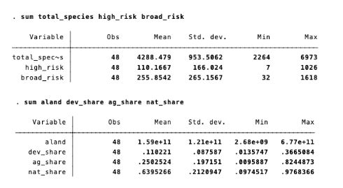
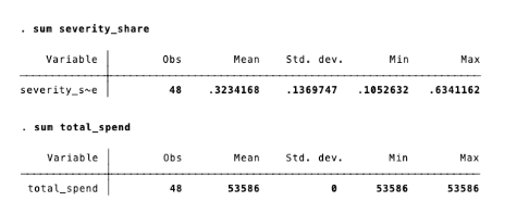
Appendix A: Summary of Key Variables in Data
Appendix B: Ecological Risk Variables Correlations in the Dataset
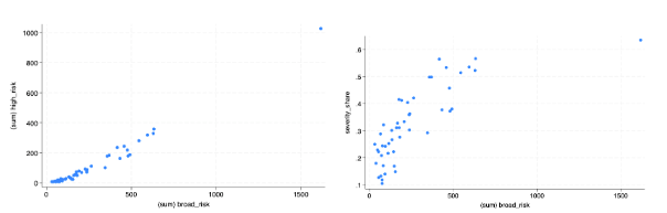
The count of high-risk species, broad risk species, and severity_share all display a positive correlation with each other.
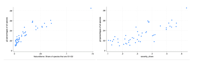
The count of species categorized as G3 (level of endangeredness) has a positive relationship to high-risk species count, and severity share variable.
Appendix C: Land Characteristics Correlations in the Dataset
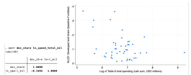
The developed land area as a share of a state’s total land area is negatively correlated with the amount of federal funding it receives for conservation.
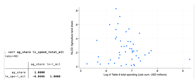
The agricultural land area as a share of a state’s total land area has a weak positive relationship with the amount of federal funding it receives for conservation.
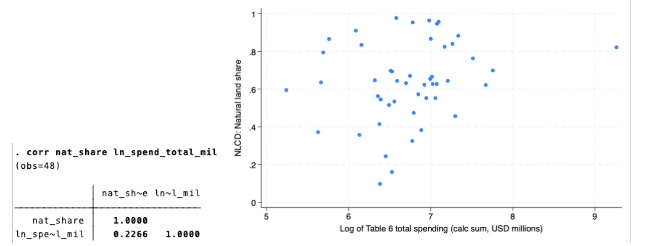
The natural land area as a share of a state’s total land area has a positive relationship with the amount of federal funding it receives for conservation.
Appendix D: Regression Outputs
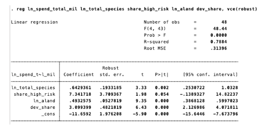
At first, we started with the most general form of regression estimation. This is consisted with 2 variables representing ecological risks, and 2 variables representing land characteristics to examine their crude OLS relationship with the spending level by each state. This is the model we’re using for interpretations. The subsequent analysis include add-ons from this model.
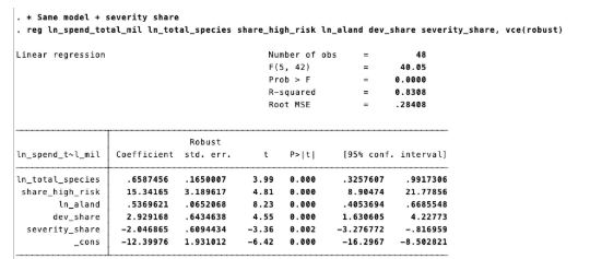
Then, after creating the severity share variable, adding it in would help the model explain for a state with, say, an overwhelming number of highly endangered species (categorized as G1 and G2), then the result shows that with a state having more of the high-risk species, they actually receive less funding, according to this model, and all variables are statistically significant at the 95% confidence level.
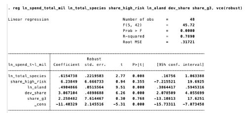
Given the counterintuitive result from the above output, the variable severity risk might underexplain the effect of G3 counts. To isolate this effect, putting only the share of G3 species for states, the regression shows that as G3 counts increase, the state gets more funding. However, this result is not statistically significant.
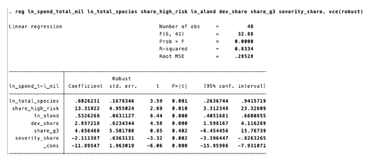
Lastly, using both severity share and share of G3 in the same model to prevent OVB bias, even though the share of G3 species counts are not statistically significant, it effectively presents the effect of G3 to the funding considerations.
Appendix E: Redistribution Results – Gaps and Amount Receivable
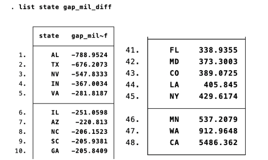
After the relocation process, the top underfunded states, based on their ecological risks and land characteristics, are listed on the left side numbered 1 ~ 10. The most “overfunded” state is California, and top overfunded states are listed in the right table.
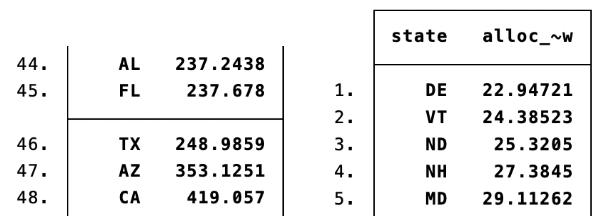
After the redistribution process, the top receivers are listed on the left side, and the lowest receivers are on the right. These reallocation results do not represent the amount of money to bring the state to its maintenance, but it’s the composite consideration of the state’s ecological and land characteristics and the redistribution of the national surplus.
Author Bio

Yusuf Khaled is a second-year Master of Public Administration student at Cornell University’s Jeb. E. Brooks School of Public Policy, concentrating on Economic and Financial Policy, and pursuing a certificate in Environmental Finance and Impact Investing. Before Cornell, he earned his bachelor’s degree in International Criminal Justice from John Jay College (CUNY), where he served as the Student Council President. He has professional experience in sustainability, housing, and public administration, including work with Implus LLC on ESG and sustainability reporting and with NYC PACT Housing on affordable housing transitions. Fluent in Bengali and conversational in Hindi and Urdu, Yusuf is passionate about advancing sustainable finance and equitable economic development.