Rigging Elections: A Spatial Statistics Analysis of Political and Unintentional Gerrymandering

Introduction

The 2016 election cycle was fraught with claims of election rigging. Though mostly unsubstantiated, there may be some truth to these claims — at least at the congressional level.

Every two years, congressional elections (or midterm elections) are held to fill seats in the House of Representatives. Unlike the president, representatives are elected based on the popular vote, meaning that the candidate who receives the most votes gets to represent their district in Congress.

By federal law, each district is required to:

• have about the same population as the other districts within the state
• allow minority voters equal opportunity to participate in the political process

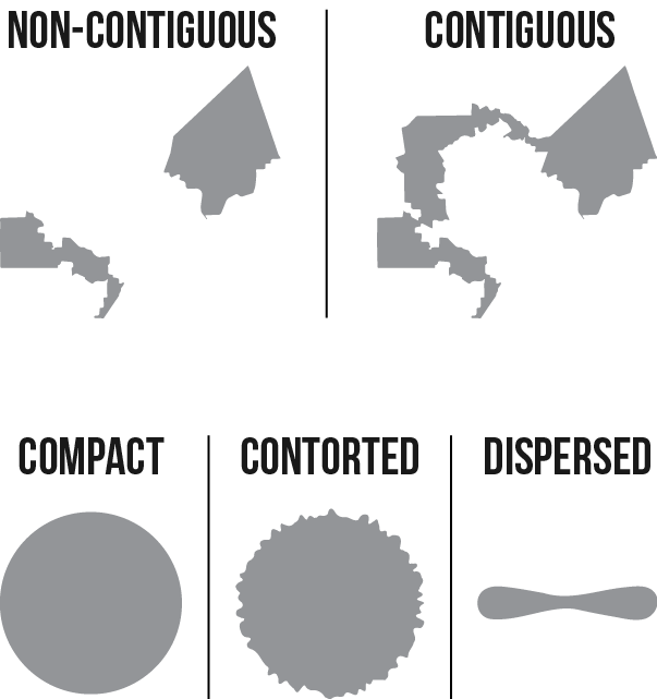
Figure 1: Requirements for district shapes.

Most states also require districts to:

• be contiguous, meaning that they must have a single, unbroken shape
• be “compact,” meaning that they should have smooth rather than contorted boundaries and should cluster around a central core, rather than dispersing outwards¹

After each decennial census, congressional districts are redrawn based on the newly updated population and demographic data. In most states, the majority party in the state legislature is tasked with redistricting, or redrawing the district boundaries.

Since congressional elections are based on popular vote, the way in which districts are drawn can impact the outcome of the election. By extension, the party in charge of redistricting has an incentive to redraw districts in order to favor their party.

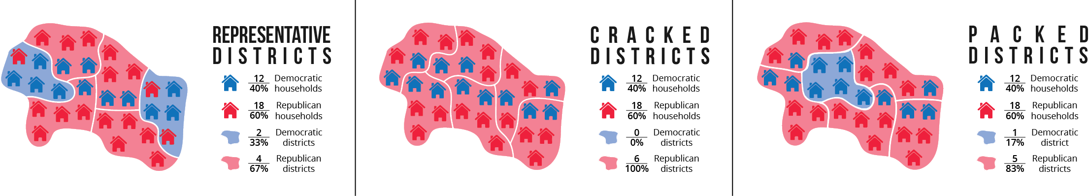
Redistricting based on political affiliation uses two strategies:

• “cracking,” or spreading like-minded voters among multiple districts in order to dilute their impact and prevent them from constituting a majority
• “packing,” or concentrating like-minded voters in a single district, thereby allowing the other party to win the remaining districts²

Figure 2: Redistricting strategies.

Redrawing congressional districts for political reasons is perfectly legal, and it is often referred to as political gerrymandering. Though the term “gerrymandering” has a markedly negative connotation, gerrymandering is only illegal when it reduces the influence of minority voters based on their race, ethnicity, or language.

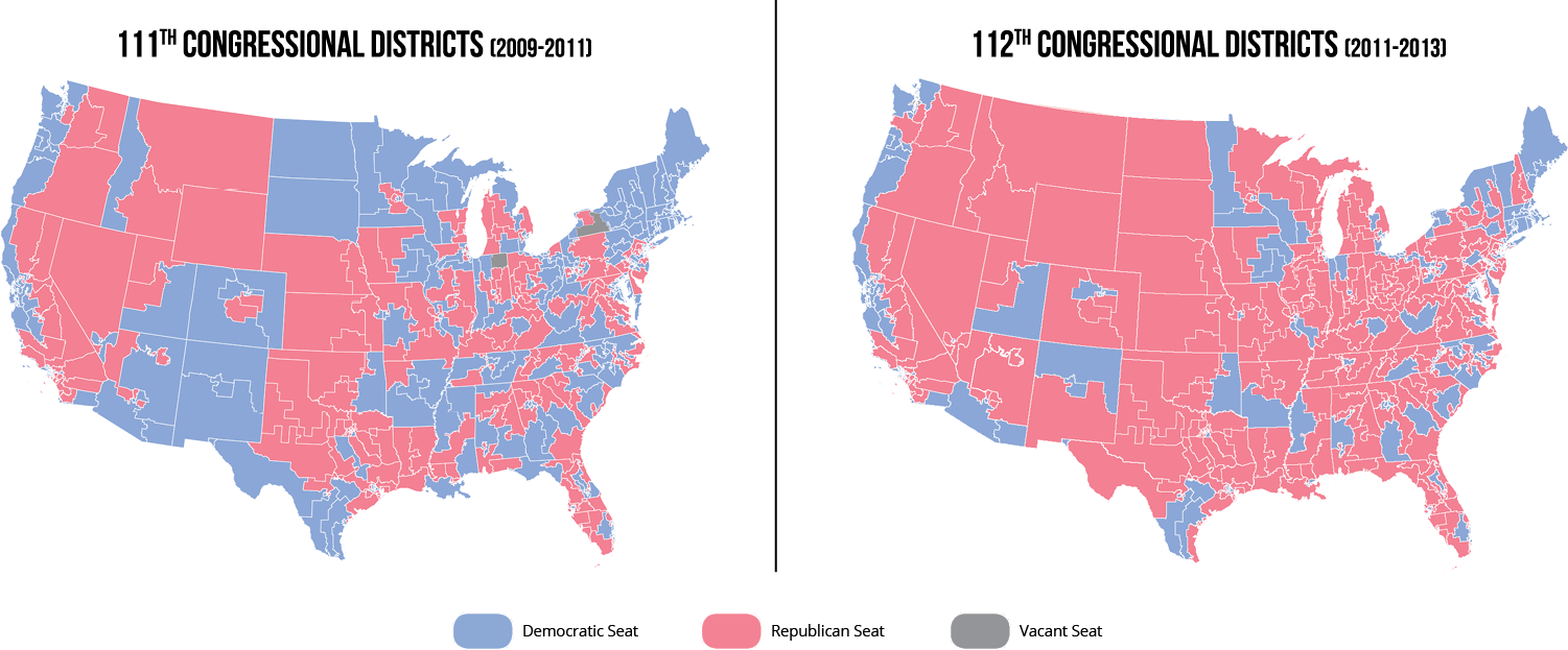
Despite the fact that political gerrymandering is technically legal, opposing parties often suggest that gerrymandering unfairly allows their opponents to win additional congressional seats. For example, after the 2010 census, Republicans were in control of approximately 60% of state legislatures and were able to redraw district boundaries in those states; during the congressional elections held later that year, the Republicans gained a majority of House seats despite the fact that Democratic candidates received more votes nationwide.³ Various media outlets and Democratic politicians have attributed this disparity to Republican gerrymandering; if Democrats won the nationwide popular vote, then Republicans must have either cracked or packed districts to dilute the influence of those Democratic voters.

Figure 3: Party control of congressional districts before and after significant Republican redistricting.

However, this argument does not consider the underlying distribution of Democratic and Republican voters. The following analysis will use geographic information system (GIS) data and spatial statistics to visualize the “natural” spatial distribution of political affiliation. Such analysis will also determine to what extent the outcome of the 2012 congressional elections were impacted by intentional political gerrymandering or the spatial pattern of voters. By using this objective, statistical approach, the resulting policy implications are intended to provide non-partisan, constructive methods for addressing bias — both intentional and unintentional — in congressional elections.

Literature Review

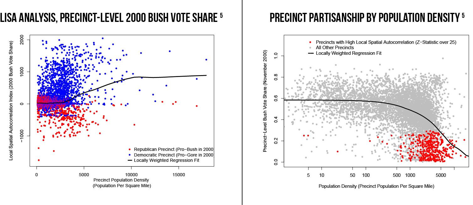
Studies have found that voters are not scattered at random — rather, they cluster near other voters with similar political preferences and party orientations.⁴ A study conducted by a team of political scientists (Chen and Rodden) determined that the probability that two randomly drawn individuals exhibit similar voting behavior is a function of the distance between their locations.⁵ Such findings suggest that voting behavior is spatially autocorrelated, meaning that individuals who live in close proximity with one another (on precinct-level scales) are more similar in political preference than those who live farther apart.

Chen and Rodden also found that the level of spatial autocorrelation differs between the two major political parties in the United States. The below left figure shows that Democratic precincts are more spatially autocorrelated (higher local spatial autocorrelation index) than Republican precincts. The below right figure also indicates that precincts with low Republican vote-shares (or more Democratic precincts) have higher population densities on average. In combination, these two patterns suggest that Democratic voters are inefficiently concentrated in large cities, while Republican voters tend to be spread more evenly throughout a state. The authors claim that this “unintentional gerrymandering” due to human geography ultimately favors Republicans.⁶

Figure 4: Statistical evidence for “unintentional gerrymandering” of Democratic voters.

Source: Chen, J. and J. Rodden. “Tobler’s Law, Urbanization, and Electoral Bias: Why Compact, Contiguous Districts are Bad for the Democrats.” 2009. http://web.stanford.edu/~jrodden/chen_rodden_florida.pdf.

Methodology

This study will attempt to determine to what extent intentional political gerrymandering — or unintentional gerrymandering due to the spatial distribution of voters — may have impacted the 2012 congressional elections. In 2012, Democrats received 48.8% of the overall popular vote in House elections, while Republicans received 47.6%. However, Republicans won 51.7% of the House seats, while Democrats won 44.9%.³

Figure 5: Difference in the number of House seats won versus the number of seats each party should have earned based on its proportion of the 2012 popular vote.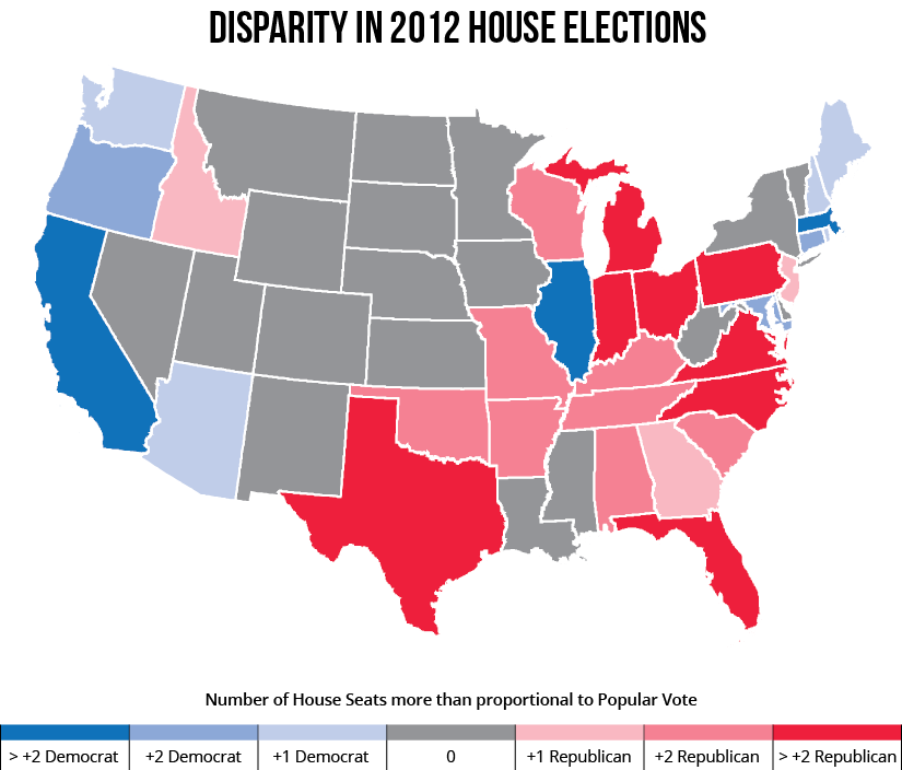

One potential cause of this disparity is that, after the 2010 census, Republicans intentionally politically gerrymandered congressional districts to dilute the impact of Democratic voters. For instance, boundaries could be drawn to pack likely-Democratic voters into relatively few districts such that Republican candidates could win the rest of the districts in a given state. Similarly, boundaries could be drawn to spread likely-Democratic voters more thinly across many districts, thereby lessening their influence in each district.

Another cause of this disparity could be the unintentional gerrymandering caused by like-minded voters, particularly Democrats, living in close proximity to one another. If Democrats have a higher degree of spatial autocorrelation than Republicans, Democratic votes might be wasted in districts where Democratic candidates already win by large margins.

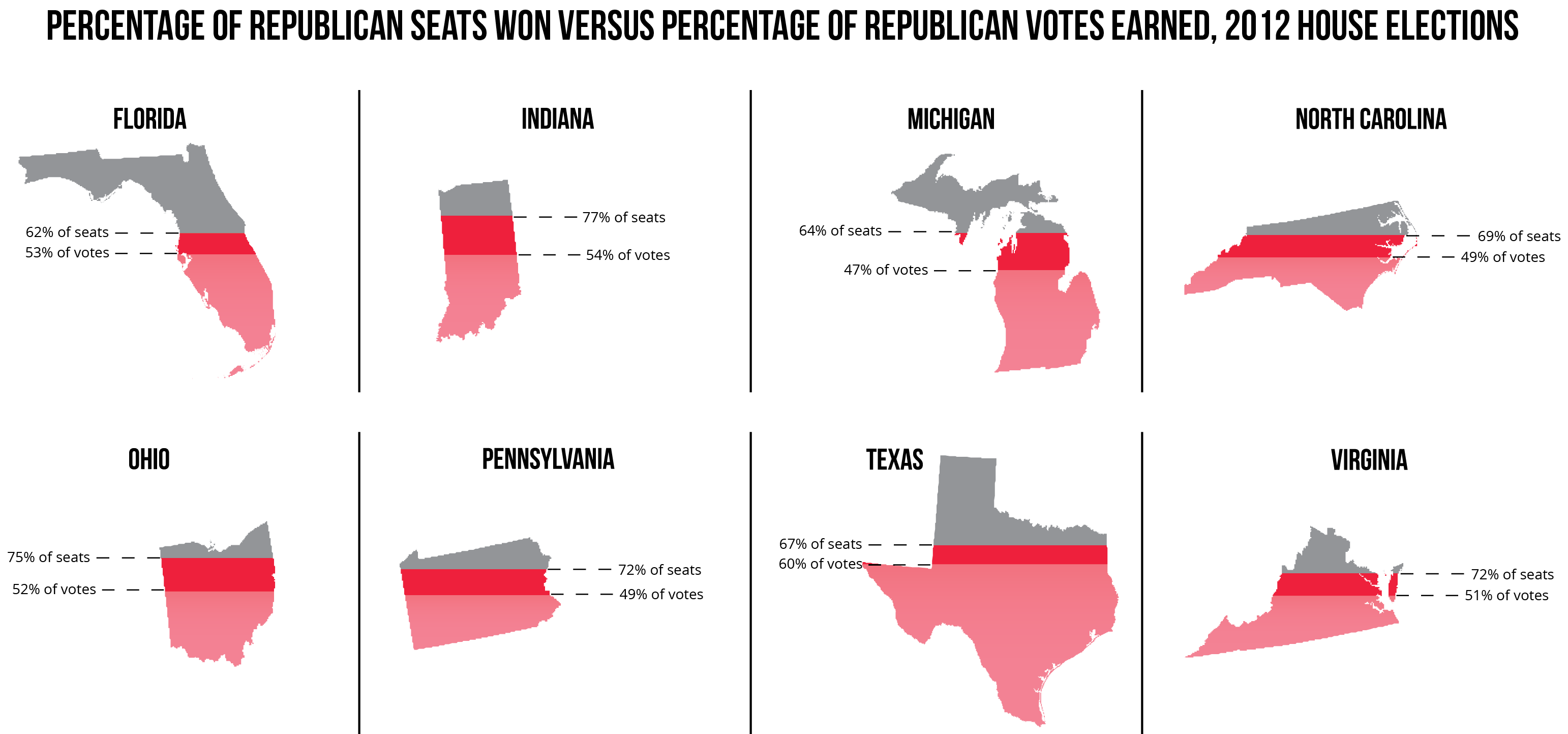
This study will be constrained to eight states where, in 2012, Republicans won at least two more seats in the House than they should have earned from their proportion of the popular vote. For instance, in Ohio, Republicans received 52% of the popular vote, which should have earned them 8 seats in the House. However, Republicans actually won 12 seats — 75% of the state’s total seats.³

These states also experienced similar results:

• Florida
• Indiana
• Michigan
• North Carolina
• Pennsylvania
• Texas
• Virginia

The states where Democrats won more House seats than they should have based on the popular vote are not included in this study because, in recent years, gerrymandering has often been attributed to or blamed on Republicans, as evidenced by recent headlines from The New York Times and The Washington Post reading “When Republicans Draw District Boundaries, They Can’t Lose”⁷ and “Republicans are so much better than Democrats at gerrymandering.”⁸ Furthermore, as shown in the previous map, more states experienced positive disparities in Republican seats rather than Democratic ones and, of those positive disparities, a larger percentage resulted in a gain of more than two additional Republican seats.

This study will explore whether political and/or unintentional gerrymandering influenced the difference between how many seats each party should have won, based on their proportion of the popular vote, and how many seats they actually won.

Figure 6: Disparity in 2012 House elections for states that won 2 or more Republican seats than they should have proportionally.

To measure the extent to which congressional districts in each of the eight states may have been politically gerrymandered, a proxy based on compactness was utilized. The Polsby-Popper measure, which determines compactness based on the ratio of the area of the district to the area of a circle with the same perimeter as the district, is a widely used method for approximating gerrymandering.⁹ Using this measure, districts with irregular boundaries (i.e. contorted districts) or elongated districts that do not encompass much territory (i.e. dispersed districts) will have low compactness scores. A district’s low compactness score may reflect intentional gerrymandering, or signal that it was drawn in a strange way so as to strategically include or exclude certain populations.

Since the Polsby-Popper formula is based on area and perimeter measurements, it is essential to use an equal-area projection when mapping in order to reduce distortion and accurately compare compactness scores across districts. This analysis used the North America Albers Equal Area Conic projection. After properly projecting the data, compactness scores for each United States congressional district in the 112th Congress were determined by calculating area and perimeter geometries for each district and subsequently calculating the districts’ Polsby-Popper measures. The 112th Congress was in session from 2011 to 2013, meaning that the 2012 House elections were conducted in these districts.

Figure 7: Various shapes and their corresponding Polsby-Popper compactness scores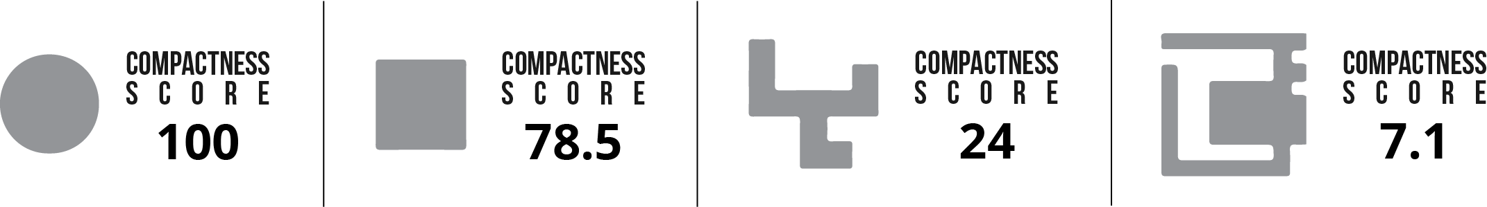

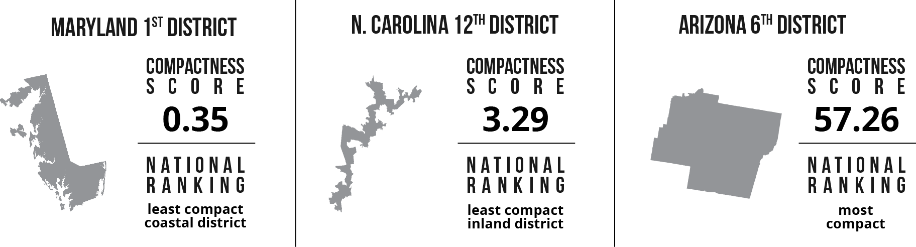
It is important to note that the Polsby-Popper measure is particularly sensitive to coastal districts, since the jagged shoreline produces very irregular boundaries. As a result, coastal districts might have slightly exaggerated compactness scores.

Figure 8: Polsby-Popper compactness scores for selected districts in the 112^th Congress.

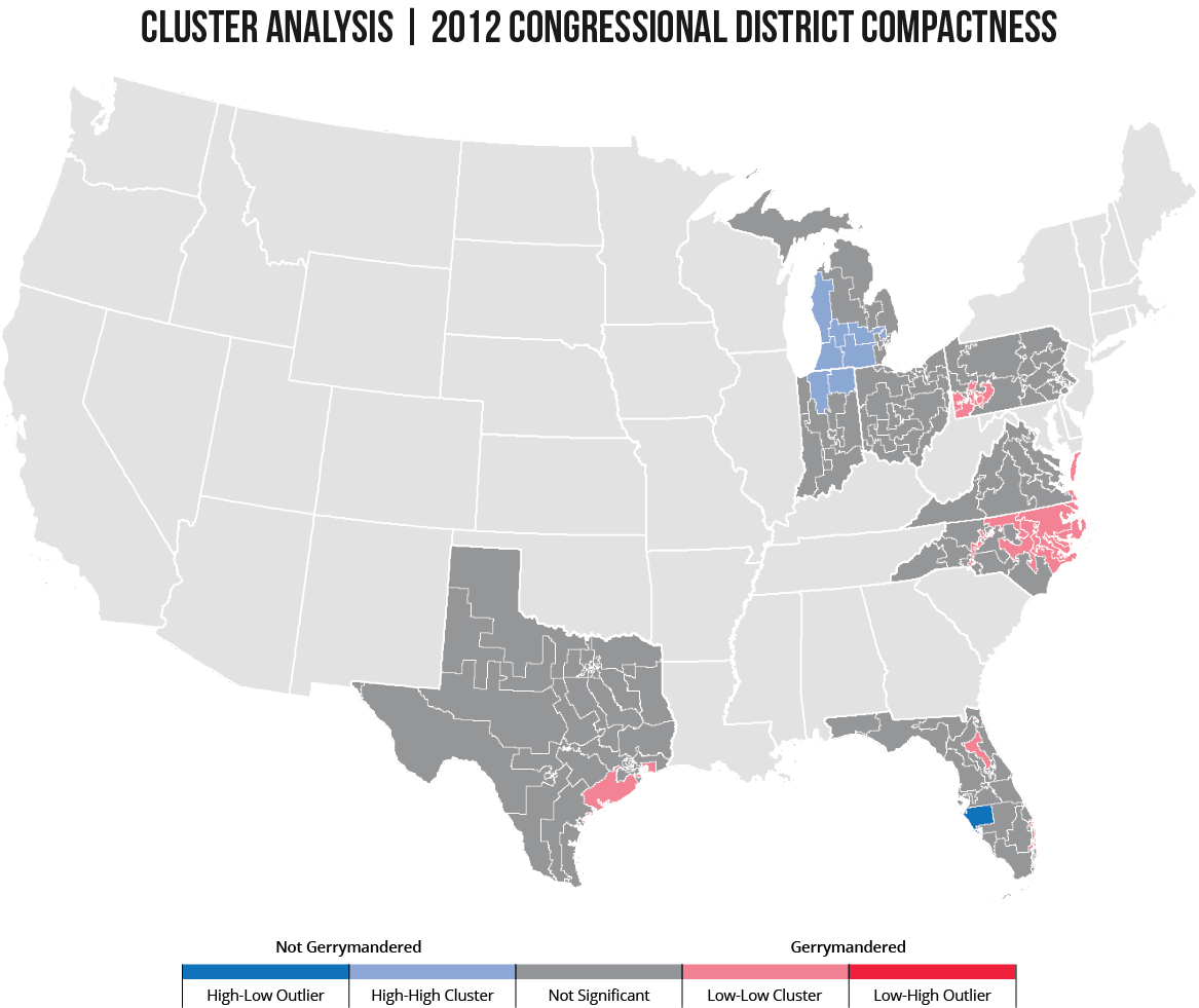
An Anselin Local Moran’s I Cluster and Outlier Analysis determined whether any congressional districts in the previously mentioned eight states had statistically significant clusters of low compactness scores (or high levels of intentional gerrymandering). The Cluster and Outlier Analysis used contiguity-edges-corners conceptualization because the shape of a district is dependent upon the coterminous boundaries of its neighbors. In other words, a district with an irregularly-shaped side will result in an adjacent district with that same irregularly-shaped side because of their coterminous relationship. As a result, highly gerrymandered districts are likely to appear as clusters.

The resulting visualization indicates areas where districts are surrounded by other districts with similarly high or low compactness scores: such spatial clustering is more pronounced than would be expected in a random distribution. The low compactness clusters are colored red to indicate a higher degree of intentional gerrymandering, while the high compactness clusters are colored blue to indicate a lower degree.

Figure 9: Statistically-significant gerrymandered districts.

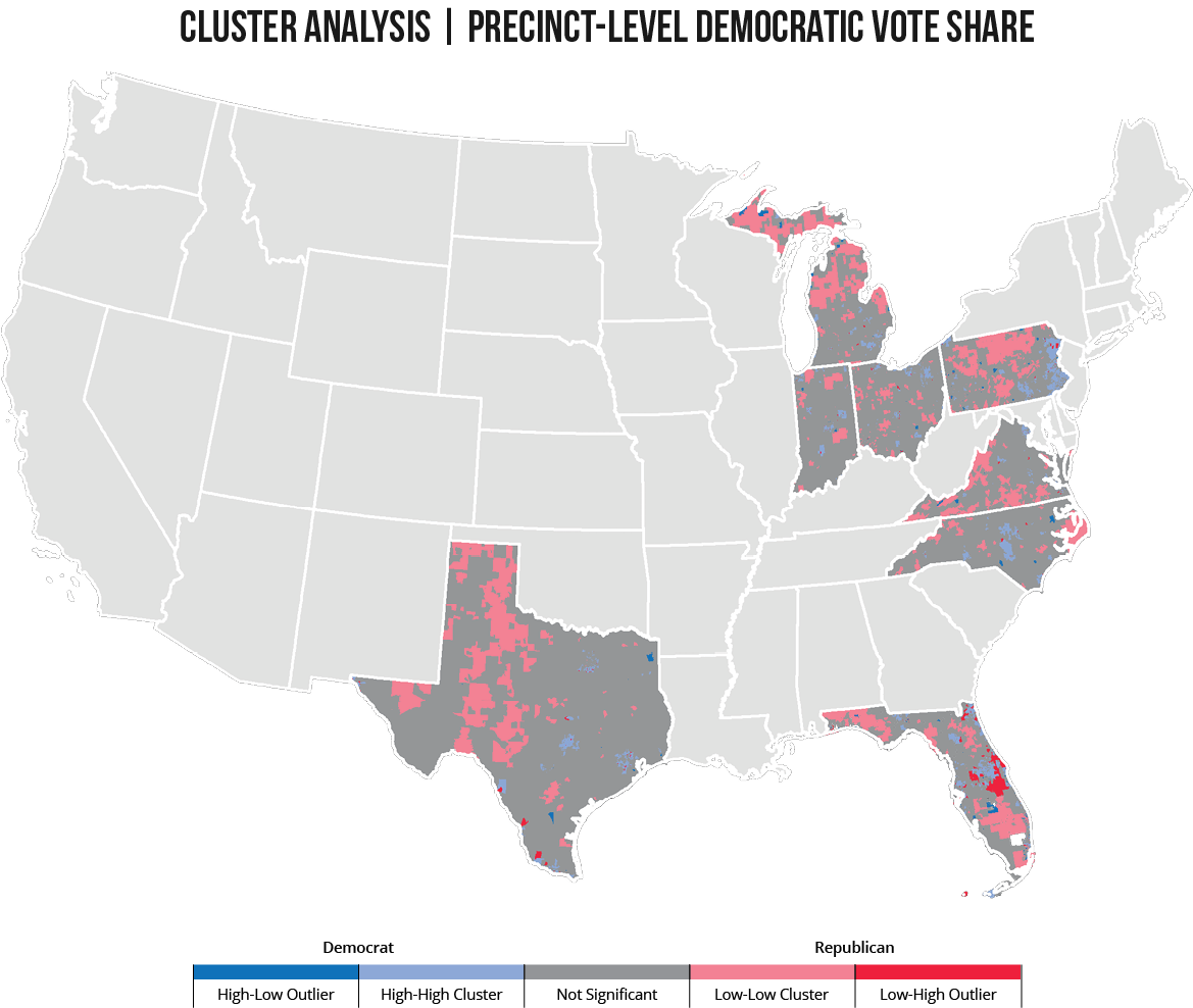
To measure the extent to which congressional districts in these eight states may have been unintentionally gerrymandered (due to Democratic voters clustering in densely-populated cities), another Anselin Local Moran’s I Cluster and Outlier Analysis was performed in order to identify clusters of “normal Democratic votes” for each precinct in the eight states. Normal Democratic votes, or NDV, uses the average Democratic vote share in previous state and presidential elections, normalized to the turnout in the 2008 presidential election, to measure how many likely-Democratic voters live in a given precinct.

NDV = (average Democratic vote share in all statewide and presidential elections from 2004 to 2008) × (2008 presidential turnout)

This cluster analysis looks at precincts because precincts are eventually aggregated into larger congressional districts. Thus, if clustering of Democratic voters exists among neighboring precincts, then the districts inclusive of these precincts will be more likely to vote Democratic, based solely on the human geography of where certain voters live.

Figure 10: Unintentional gerrymandering due to party clustering.

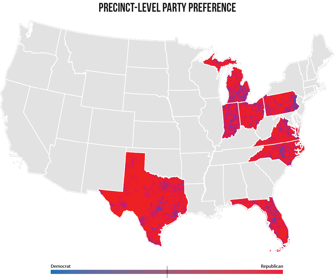
After performing the cluster analysis on normal Democratic votes, the square of the Local Moran’s I (LMI) value for each statistically significant precinct was used as the extrusion value, or the height to which each precinct was upwardly extended in three-dimensional space. Since the LMI is based on normal Democratic votes, a positive LMI is indicative of clustering of Democratic voters, whereas a negative LMI is indicative of clustering of Republican voters. (For this analysis, political preference was considered binary; voters are either Democrats or Republicans.) Squaring these LMI values ensures that all precincts are extruded in the same direction. This means that the relative extrusion heights for each precinct can be used to compare the degree to which either Democratic or Republican voters are clustered. The higher the extrusion, the more clustering of a specific political preference.

By overlaying political preference on these extrusions, it is possible to see where certain political preferences are clustered (based on color) and to what extent they are clustered (based on height of extrusion). To display party preference, the NDV for each precinct was symbolized using natural breaks and color ramped from red to blue. Precincts that are red vote strongly Republican (low NDV) and precincts that are blue vote strongly Democratic (high NDV), while precincts that are purple-ish are less partisan.

Figure 11: Spatial distribution of political preference.

To reiterate, the objective of this analysis is to determine whether states that won proportionally more Republican seats in the 2012 House of Representatives than they should have based on the popular vote did so as a result of intentional and/or unintentional gerrymandering.

Figure 12: Process used to create the following maps.

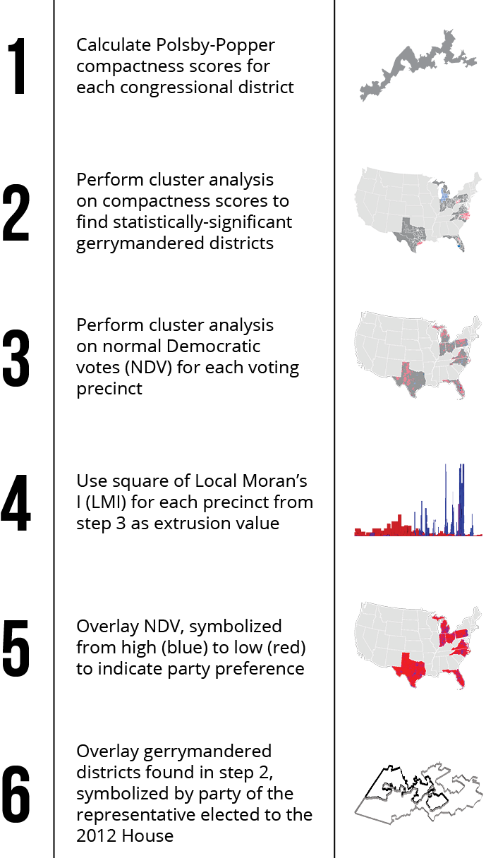
By adding the gerrymandered districts (as determined by the cluster analysis on the congressional district compactness scores) to the extruded maps for each state, it is possible to see where gerrymandered districts are located in relation to clusters of voters. Clusters of voters located immediately outside gerrymandered districts may have been purposefully excluded to improve the opposing party’s odds of winning. Contrarily, clusters of voters located within gerrymandered districts may have been packed to dilute their influence elsewhere.

If no clusters of gerrymandered districts exist in a state, the reason for the disproportionate number of Republican seats must, by process of elimination, result from intense clustering of Democratic voters, as indicated by high, blue extrusions.

However, if gerrymandered districts do exist in a state, the disparity in seats versus votes may be attributed to intentional gerrymandering alone or to a combination of intentional and unintentional gerrymandering.

In the following maps, gerrymandered congressional districts that elected a Democrat to the House in 2012 are outlined in white, while districts that elected a Republican are outlined in black.

Analysis

Two main categories became evident after performing this analysis for each state. The first category consists of states showing some degree of both intentional and unintentional gerrymandering. These include:

• Florida
• North Carolina
• Pennsylvania
• Texas

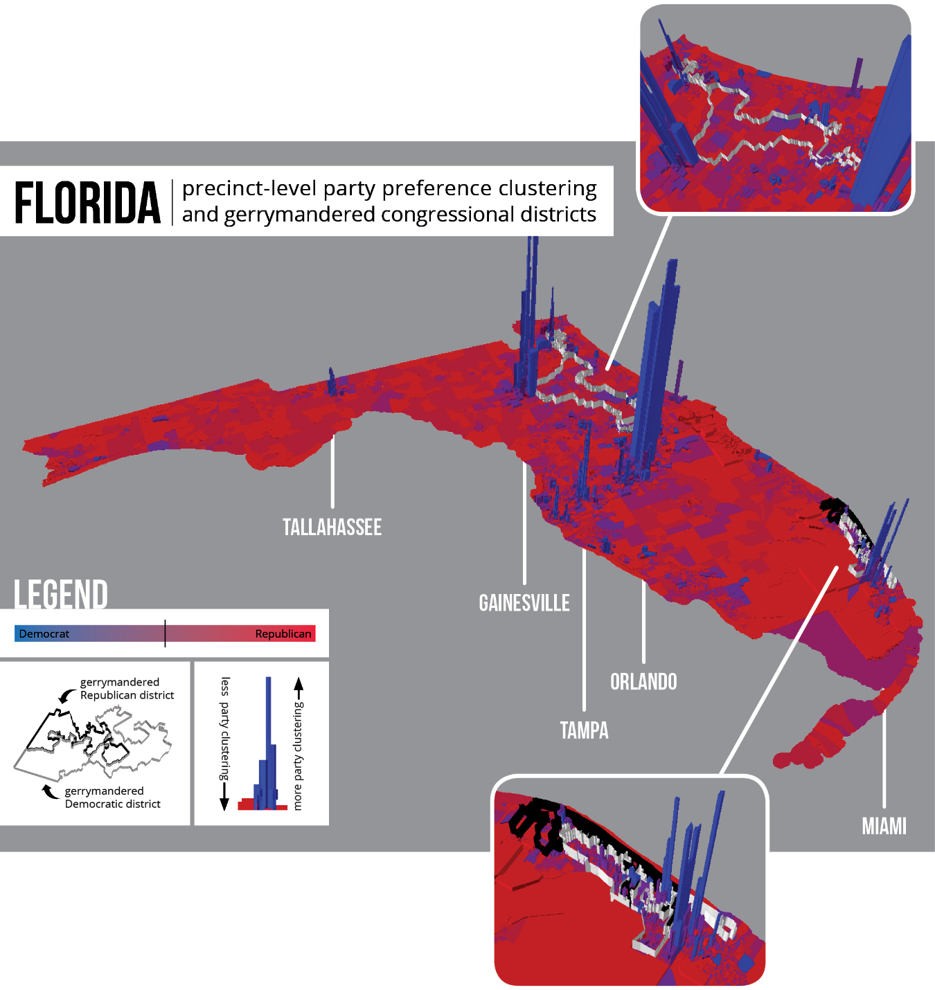
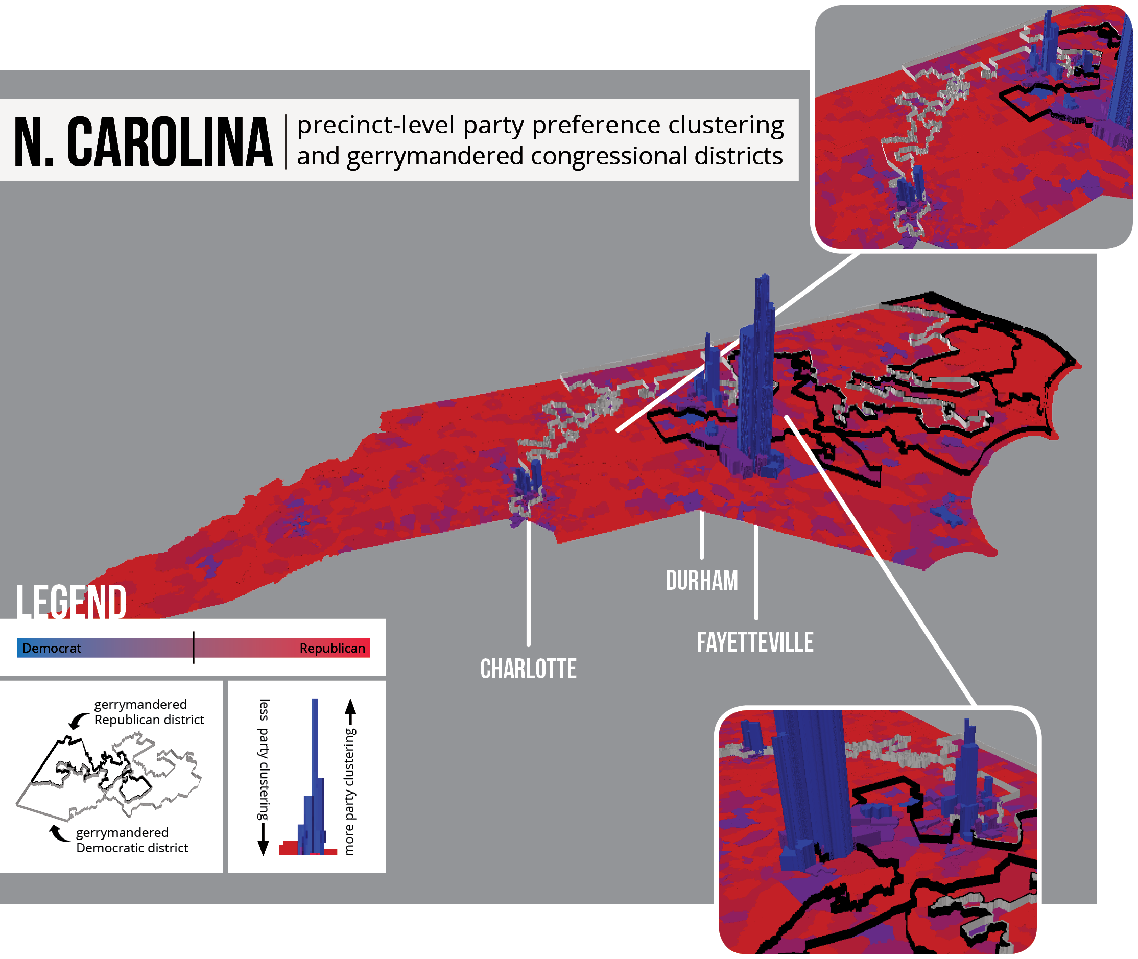
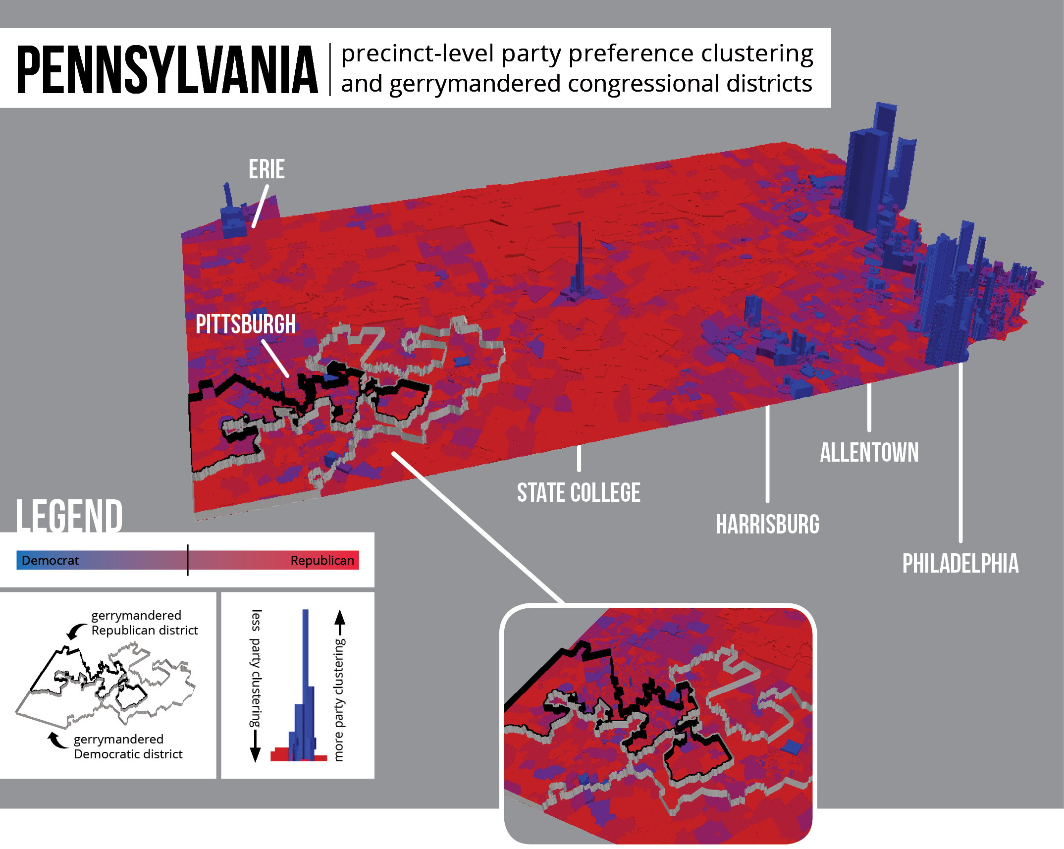
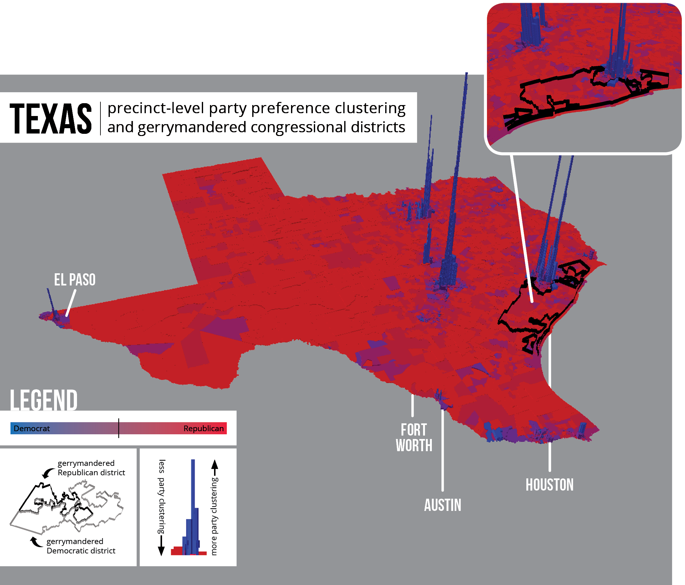
For each of these states, the previous cluster analysis on compactness scores returned statistically significant low clusters, a situation used in this analysis as a proxy for intentional gerrymandering. In Florida, two of the four districts returned in the cluster analysis were deemed unconstitutional by the Florida Supreme Court.¹⁰ The same ruling was found for two statistically significant districts in North Carolina.¹¹ The low clusters in Pennsylvania, though not deemed unconstitutional, are located near Pittsburgh, a city that exhibits much less clustering by party preference than does a city like Philadelphia. Thus, gerrymandering in this less partisan area might secure otherwise contested seats. The significant cluster in Texas was also not deemed unconstitutional, but it does seem to contort its boundaries to strategically exclude the adjacent, largely-Democratic city of Houston.¹²

The presence of these statistically significant low clusters and the fact that some of these districts have subsequently been deemed unconstitutional indicate that some sort of intentional gerrymandering impacted the House elections in these states in 2012.

However, each state also has high blue extrusions located in large cities. These extrusions suggest extreme clustering of Democrats in densely-populated cities, a situation used in this analysis as a proxy for unintentional gerrymandering. While Republican preference is spread across larger areas, Democratic preference is constrained to cities. When Democrats cluster in this way, they essentially waste votes in areas that are already highly Democratic. Therefore, these states exhibit some level of both unintentional and intentional gerrymandering.

Map 1: Florida exhibits both unintentional and intentional gerrymandering.

Map 2: North Carolina exhibits both unintentional and intentional gerrymandering.

Map 3: Pennsylvania exhibits both unintentional and intentional gerrymandering.

Map 4: Texas exhibits both unintentional and intentional gerrymandering.

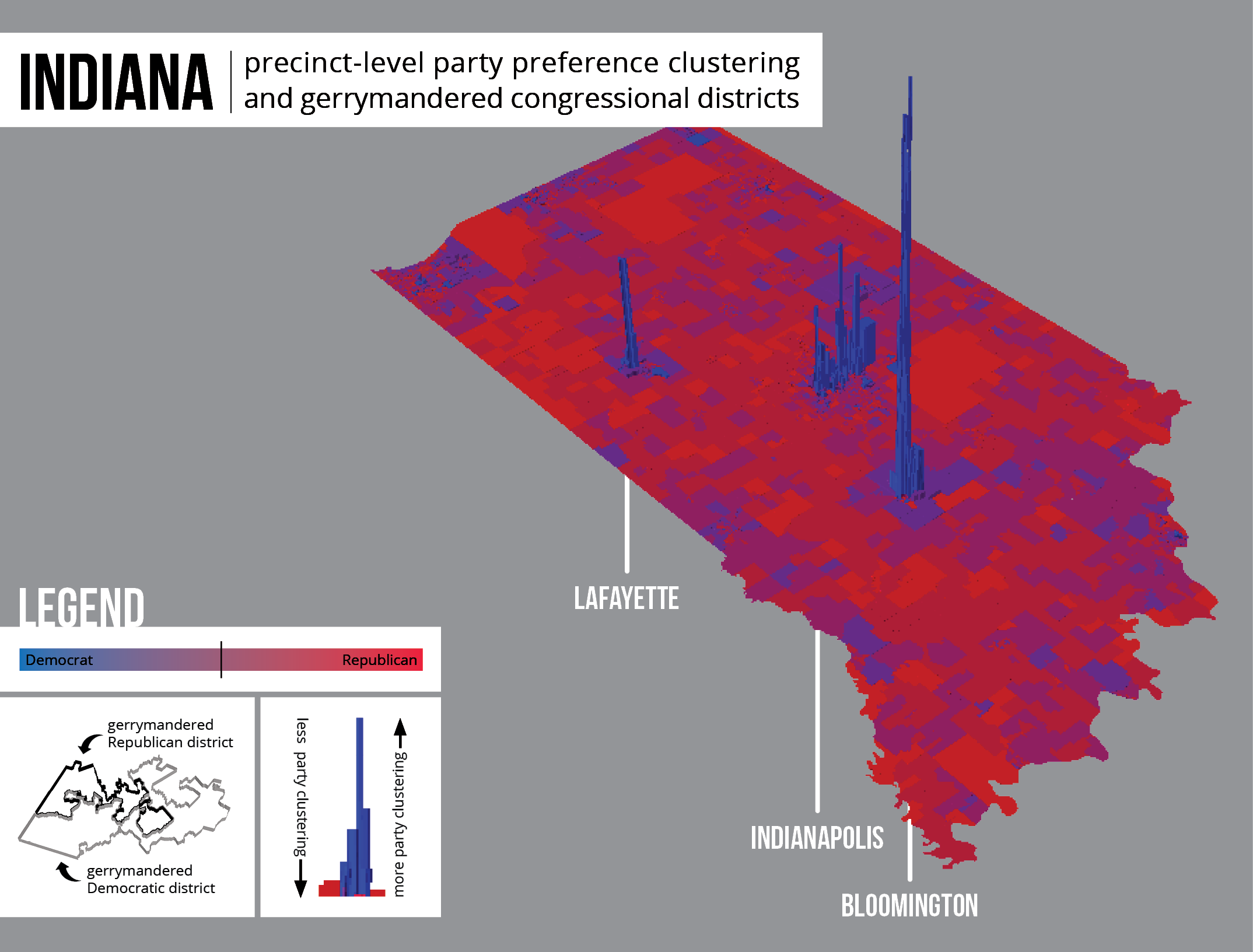
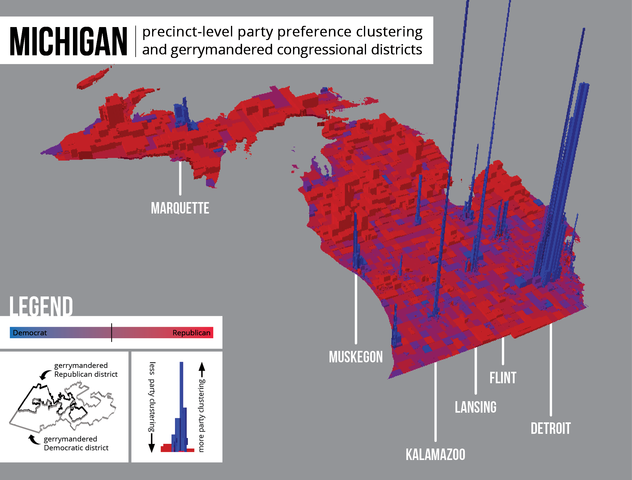
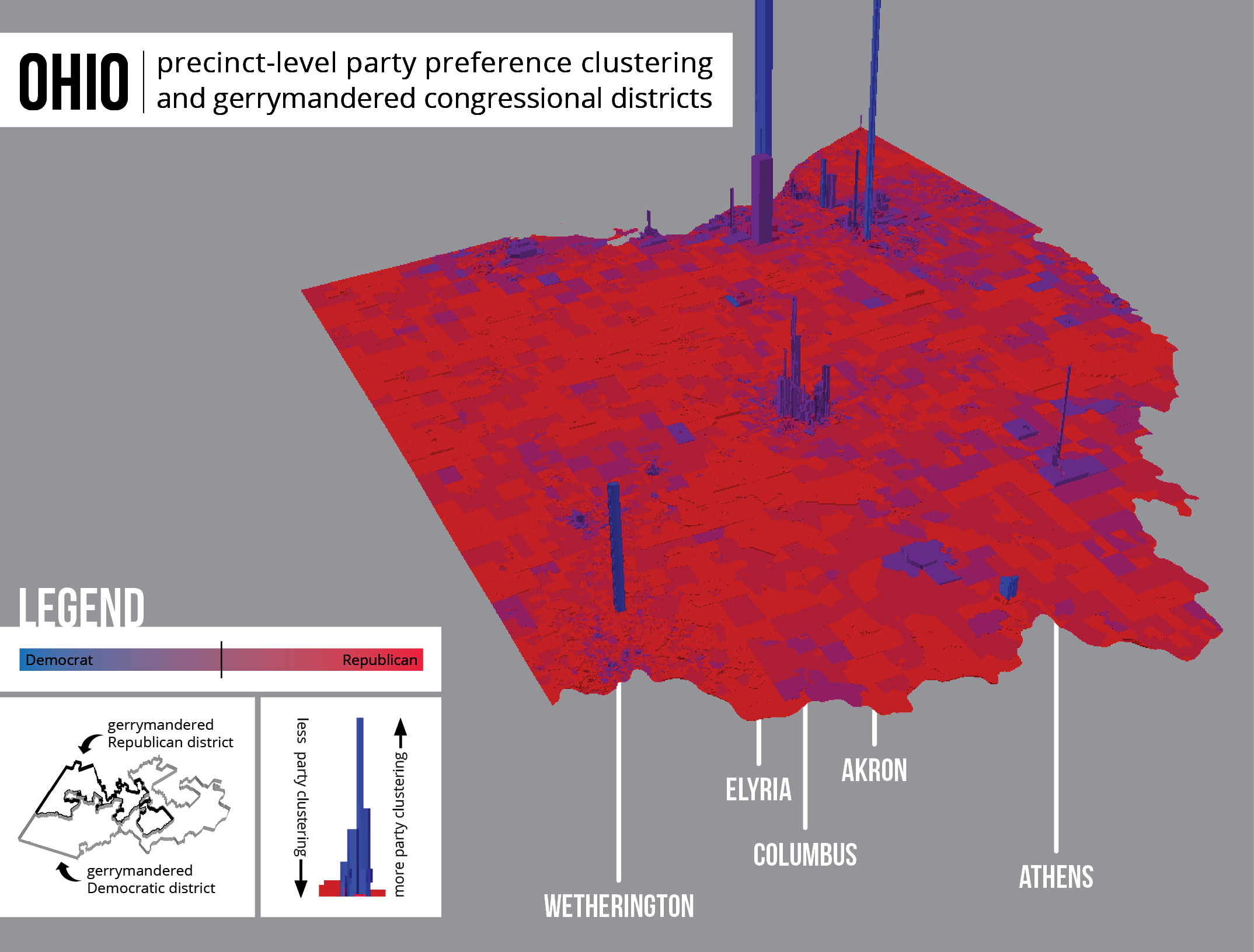
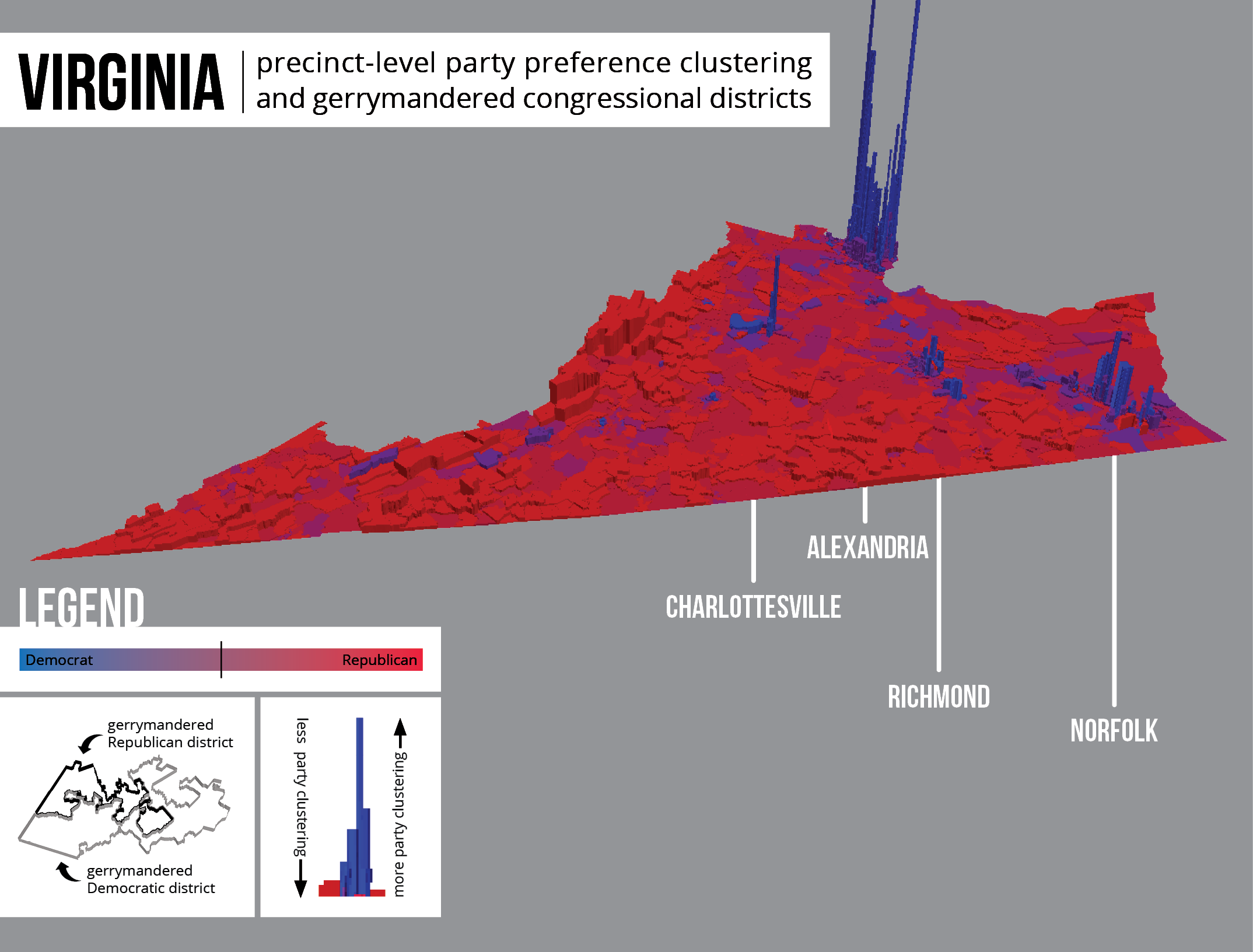
The second category showed only unintentional gerrymandering and included the following states:

• Indiana
• Michigan
• Ohio
• Virginia

For each of these states, the cluster analysis on compactness scores did not return any statistically significant clusters. Thus, by process of elimination, it can be said that Republicans received more seats in these states than they proportionally should have due to the spatial distribution of voters, or unintentional gerrymandering.

Map 5: Indiana exhibits only unintentional gerrymandering.

Map 6: Michigan exhibits only unintentional gerrymandering.

Map 7: Ohio exhibits only unintentional gerrymandering.

Map 8: Virginia exhibits only unintentional gerrymandering.

Conclusions

From this analysis, it is clear that political preference is spatially autocorrelated — voters who live closer to each other are more likely to have the same political preference. This is especially true in Democratic precincts, which have much greater Local Moran’s I values than Republican precincts (as shown by the high blue extrusions in the previous maps). While Democrats are highly clustered in large, densely-populated cities, Republicans are scattered more evenly throughout rural and suburban areas. This results in what Chen and Rodden term “unintentional gerrymandering” in which one party’s voters are more clustered than those of the opposing party due to residential patterns.⁶

Most often, unintentional gerrymandering produces a pro-Republican bias because surplus Democratic votes are “wasted” in cities (and districts) that are already heavily Democratic. If these votes were more evenly distributed among rural districts, then Democrats might be more competitive in these often-Republican districts. As shown by the previous maps, Republican precincts exhibit little to no clustering of political preference (i.e. lower extrusions), meaning that districts composed of these precincts are not strongly partisan in either direction. Despite the fact that these rural districts are less partisan than urban districts, they often tend Republican because Democratic votes are clustered in cities.

In this analysis, unintentional gerrymandering was determined to be a probable factor in the disparity between Republican seats and the proportion of Republican votes, especially in states without statistically significant gerrymandered districts — states like Indiana, Michigan, Ohio, and Virginia. The fact that such disparities exist in states without gerrymandered districts signals that the tendency to conflate observed electoral bias with political gerrymandering might be inappropriate.

The typical explanation for disproportionate representation in the House is political or racial gerrymandering by the party in control of the redistricting process, thus suggesting that politicians crack or pack congressional districts in order to favor their party. However, this and other analyses have shown that unintentional gerrymandering caused by the spatial patterns of human geography may play a larger part in electoral bias than is commonly thought.⁶ Those who blame intentional gerrymandering for disproportionate representation in the House often advocate for reforms that they attest would prohibit political gerrymandering by enforcing objective criteria like compactness and contiguity. When such criteria are imposed on districts without considering underlying political preference, studies have shown that districts continue to have a pro-Republican bias even in the absence of intentional gerrymandering.⁶

Furthermore, districting regulations that require each district to be of equal population size will inevitably create small and likely-Democratic districts around densely-populated cities, while creating much larger and less partisan rural districts. Thus, the movement for non-partisan redistricting committees seems rather baseless, since partisan districts result naturally from the spatial pattern of political preference.¹³ In fact, these ostensibly apolitical districting regulations themselves might contribute to, rather than reduce, electoral bias. Studies that ran automatic redistricting simulations have found that schemes that prioritize compactness will produce a bias against whichever party is clustered in cities.⁵

Policy Implications

This analysis found that bias in the outcomes of congressional elections can result solely from the spatially dependent patterns of human geography. These findings suggest that, when the Supreme Court rules on partisan gerrymandering in 2017, it must recognize that apolitical regulations like compactness, which attempt to reduce intentional gerrymandering, will still result in unintentional gerrymandering regardless.¹⁴ Islands of blue surrounded by seas of red will persist, thereby maintaining disproportionate representation in the House.

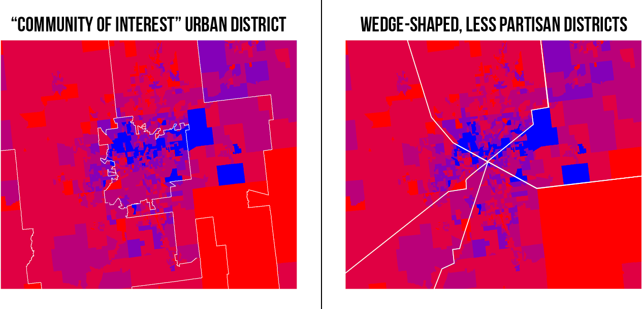
Redistricting regulations might, therefore, benefit from the consideration of the spatial patterns of political preference. Some suggest that urban districts should be drawn in wedge-like shapes that extend outward from a city to include rural areas of dissimilar political preference.¹⁵ Others claim, however, that such districts would break apart “communities of interest” — or groups with similar social, cultural, racial, or economic interests — which many states require to be preserved whenever possible.¹ As shown in this analysis, Democratic communities of interest often cluster in cities while rural areas are more often Republican; creating wedge-shaped districts that extend outward from city centers to rural areas would encompass a more even mixture of Democrats and Republicans. These districts would reduce partisanship and increase competitiveness, but would also separate communities of interest. The Court will ultimately need to decide which measures (i.e. compactness, preserving communities of interest, competitiveness) are most consequential and establish well-defined (rather than the existing vague) standards for achieving appropriate districts.

Figure 13: Different methods for creating urban districts.

This issue warrants further research to determine empirically the extent to which observed electoral bias is a result of political or unintentional gerrymandering. If the effects of each type of gerrymandering are quantifiable and distinguishable, then policies can be more appropriately tailored to address both intentional political and unintentional spatial gerrymandering.

Bibliography

1. Levitt, Justin. “Where are the lines drawn?” All About Redistricting. http://redistricting.lls.edu/where.php.
2. Azavea. Redrawing the Map on Redistricting. 2010. http://cdn.azavea.com/com.redistrictingthenation/pdfs/Redistricting_The_Nation_White_Paper_2010.pdf.
3. ProPublica. House Seats vs. Popular Vote. 2012. http://projects.propublica.org/graphics/seats-vs-votes.
4. Kendall, M.G. and A. Stuart. “The Law of Cubic Proportions in Electoral Results.” British Journal of Sociology 1(3): 183-96. 1950.
5. Chen, J. and J. Rodden. “Tobler’s Law, Urbanization, and Electoral Bias: Why Compact, Contiguous Districts are Bad for the Democrats.” 2009. http://web.stanford.edu/~jrodden/chen_rodden_florida.pdf.
6. Chen, J. and J. Rodden. “Unintentional Gerrymandering: Political Geography and Electoral Bias in Legislatures.” Quarterly Journal of Political Science 8: 239-69. 2013. http://www-personal.umich.edu/~jowei/florida.pdf.
7. Wagner, Alex. “When Republicans Draw District Boundaries, They Can’t Lose. Literally.” The New York Times. 2016. http://www.nytimes.com/2016/06/26/books/review/rated-by-david-daley.html.
8. Ingraham, Christopher. “Republicans are so much better at gerrymandering than Democrats.” The Washington Post. 2017. http://www.washingtonpost.com/news/wonk/wp/2017/06/06/republicans-and-democrats-both-try-to-gerrymander-but-only-one-of-them-is-any-good-at-it/?utm_term=.1478040748e3.
9. McGlone, Daniel. “Measuring District Compactness in PostGIS.” Azavea. July 11, 2016. http://www.azavea.com/blog/2016/07/11/measuring-district-compactness-postgis/.
10. Klas, Mary Ellen. “Court Orders Florida’s Congressional Districts Redrawn.” Miami Herald. 2015. http://www.miamiherald.com/news/politics-government/article26860765.html.
11. Walsh, Mark. “Supreme Court Considers Challenges to Racial Gerrymandering.” ABA Journal. 2016. http://www.abajournal.com/magazine/article/scotus_redistricting_racial_gerrymandering.
12. “Court Strikes Down Texas’ GOP-drawn Congressional Map for Racial Gerrymandering.” Daily Kos. 2017. http://www.dailykos.com/story/2017/3/14/1642985/-Morning-Digest-Court-strikes-down-Texas-GOP-drawn-congressional-map-for-racial-gerrymandering.
13. Petry, Eric. “Redistricting Reform Gains Momentum in 2016.” Brennan Center for Justice. 2016. http://www.brennancenter.org/blog/redistricting-reform-gains-momentum-2016.
14. Grofman, Bernard. “The Supreme Court will Examine Partisan Gerrymandering in 2017. That Could Change the Voting Map.” The Washington Post. 2017. http://www.washingtonpost.com/news/monkey-cage/wp/2017/01/31/the-supreme-court-will-examine-partisan-gerrymandering-in-2017-that-could-change-the-voting-map/?utm_term=.426156d31895.
15. Rodden, J. “The Geographic Distribution of Political Preferences.” Annual Review of Political Science 13: 321-40. 2010. http://web.stanford.edu/~jrodden/annurev.polisci.12.031607.pdf.

Data Sources

1. 111th Congressional Districts Boundaries, ESRI Data and Maps, http://www.arcgis.com/home/item.html?id=4e2e8b04eac543429d3611b67da1e198.
2. 112th Congressional Districts Boundaries, ESRI Data and Maps, http://www.arcgis.com/home/item.html?id=a5e84bcbbd9b44688d20a1a48e03723d.
3. United States Boundaries, U.S. Census Bureau Cartographic Boundary Shapefiles – States, http://www.census.gov/geo/maps-data/data/cbf/cbf_state.html.
4. Florida Precinct-Level Election Data, Harvard Election Data Archive, http://dataverse.harvard.edu/dataset.xhtml?persistentId=hdl:1902.1/16797.
5. Indiana Precinct-Level Election Data, Harvard Election Data Archive, http://dataverse.harvard.edu/dataset.xhtml?persistentId=hdl:1902.1/16050.
6. Michigan Precinct-Level Election Data, Harvard Election Data Archive, http://dataverse.harvard.edu/dataset.xhtml?persistentId=hdl:1902.1/15964.
7. North Carolina Precinct-Level Election Data, Harvard Election Data Archive, http://dataverse.harvard.edu/dataset.xhtml?persistentId=hdl:1902.1/15965.
8. Ohio Precinct-Level Election Data, Harvard Election Data Archive, http://dataverse.harvard.edu/dataset.xhtml?persistentId=hdl:1902.1/15844.
9. Pennsylvania Precinct-Level Election Data, Harvard Election Data Archive, http://dataverse.harvard.edu/dataset.xhtml?persistentId=hdl:1902.1/16389.
10. Texas Precinct-Level Election Data, Harvard Election Data Archive, http://dataverse.harvard.edu/dataset.xhtml?persistentId=hdl:1902.1/15890.
11. Virginia Precinct-Level Election Data, Harvard Election Data Archive, http://dataverse.harvard.edu/dataset.xhtml?persistentId=hdl:1902.1/15551.
12. House Seats vs. Popular Vote (2012) Data, ProPublica, http://projects.propublica.org/graphics/seats-vs-votes.

Jeanette Petti

Jeanette Petti is a senior in Cornell's urban and regional planning program, with additional interests in architecture and design. She currently works as a consultant at a planning firm in her hometown of Rochester, New York. After graduation, she intends on pursuing a master's degree in regional planning.

View all posts