
Abstract: The Supreme Court’s ruling in Citizens United v. Federal Election Commission has received much of the blame for the extraordinary amounts of money in American politics. While this decision certainly allowed for greater amounts of money in politics, Citizens United was the culmination of a larger causal trend, not the catalyst. From 1972 to 2008, prior to the ruling on Citizens United, the total spending in presidential campaigns increased by roughly 1,220%, with a 98% increase occurring from 2004 to 2008 alone.[1] I argue, rather, that growing economic inequality – rather than Citizens United – is the root cause of the vast influence of money in politics that we see today. Examining this link between inequality and campaign finance, I find that there exist strong correlations between the incomes of top earners and money in politics, both at the national and state level. Assessing these findings, I then present the implications for policy and avenues for future research.
When questioned about his motivations for robbing banks, Willie Sutton, the notorious American bank robber, allegedly responded, “Because that’s where the money is.” Though simplistic, this logic – since referred to as “Sutton’s Law” – serves as a timeless reminder to always explore the obvious before contemplating alternative explanations. When it comes to the study of campaign finance and the causes of money in politics, one need only to follow Sutton’s approach: go where the money is. Since the 1970s, the richest 1% of Americans has claimed an increasing share of the total income in the United States, while the bottom 99% of earners have seen their share decrease substantially.[2] Yet, despite the majority of Americans accounting for a dwindling share of the total income, the amount of spending in national elections – financed primarily through campaign contributions – has increased exponentially over the same period.[3] The conventional wisdom often blames the Supreme Court’s ruling in Citizens United v. Federal Election Commission (hereafter “Citizens United”) for this phenomenon. The logical first step in determining where the money is coming from, however, should be to look where the money is: the wealthiest Americans. While Citizens United may have allowed for nearly endless amounts of money to flow into the political system, evidence suggests that it may be the culmination of a larger causal trend than the cause itself.
This analysis investigates the influence of income inequality on campaign spending and contributions in the United States – at both the national and state levels – in the decades prior to Citizens United. By extending the analysis but briefly into the Citizens United era, this study controls for any spending distortions that the ruling caused. The following analysis is broken down into four sections. First, some necessary context is provided by briefly observing the trend of growing income inequality in the United States since the 1970s. In particular, I trace the income shares of the top 1% and the bottom 99% over a period from 1970 to 2012. Leveraging various academic studies, I then observe trends in campaign spending – presidential and congressional – during each presidential election cycle from 1972 to 2008, and demonstrate how they significantly correlate with the income share of the top 1%. In addition, simple linear regressions are conducted to test each correlation for causation and robustness. In the next section, the same correlations are examined at the state level, and find that states with larger income shares of the top 1% give more campaign contributions – per capita – than more equal states. In the third section, counterarguments are addressed and policy options are explored.
It is important to note that the intention of this article is not to demonize the wealthiest Americans or to suggest in any way that their political involvement is synonymous with rent seeking. Wealthy individuals – like any other American – have every right to participate in the political process. This article, rather, demonstrates that when income inequality grows, it provides the wealthiest Americans with the ability to provide disproportionate amounts of campaign contributions – thus leading to more money in politics and greater political influence.
Campaign Finance in the Shadow of Economic Inequality
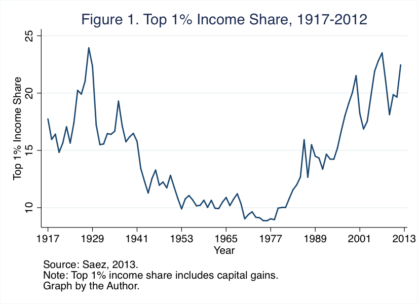
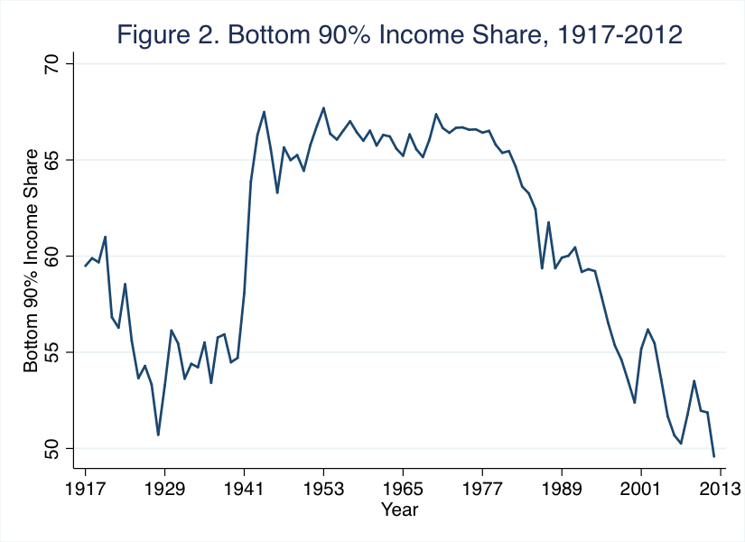
Throughout the 20th century, the income share of the wealthiest top 10% of Americans has fluctuated from 40 and 45% during the interwar period, down to roughly 30% immediately following World War II, and eventually flattening out from roughly 31 to 35% upon the 1970s.[4] During the 1970s, however, this trend began to reverse – and dramatically so – with the wealthiest Americans claiming a significantly greater share of income. Fast-forward to 2012 and the top 10% of Americans accounted for roughly 48% of total income, with 20% going to the top 1% alone.[5] These figures are lifted even further – to roughly 50% and 22%, respectively – after the inclusion of income earned from capital gains.[6] This trend among the top 1% of earners is displayed graphically in Figure 1, which charts the data compiled by Emmanuel Saez. By comparison, the bottom 90% of earners have seen their income share – displayed in Figure 2 – decrease substantially, falling from roughly 67% in 1970 to approximately 50% in 2012.[7] Essentially, the wealthiest Americans are claiming a larger share of income while the vast majority account for a decreasing share.
The implications of these income trends transcend the size of a paycheck. As Richard Wilkinson and Kate Pickett have shown, higher levels of economic inequality can have implications for the maintenance of a strong society, from social cohesion to mental and physical health.[8] Income inequality also often translates into political inequality. To see why this can be problematic, recall political scientist Robert Dahl, who famously questioned, “In a political system where nearly every adult may vote but where knowledge, wealth, social position, access to officials, and other resources are unequally distributed, who actually governs?”[9] Wealthier, more educated citizens are more likely to have well-formulated preferences, more likely to vote, more likely to contact politicians, and more likely to contribute time and energy to political campaigns.[10]
Growing income inequality stands to intensify this political dynamic. As more income flows to those at the top of the distribution, they should – in theory – become even further empowered to wield influence over the political system. The primary channel of this influence is campaign finance – donations to candidates seeking or maintaining political office. Some academic studies have found that this influence yields political results. Larry Bartels, a political scientist at Princeton, examined the voting behavior of U.S. senators and found them to be significantly more responsive to wealthy constituents than middle-income constituents, while statistically unresponsive to constituents in the bottom third of the income distribution.[11] Moreover, this disproportion in political responsiveness may cause this disparity to be self-reinforcing. As Nobel prize-winning economist Joseph Stiglitz describes:
“Those who turn out to vote are those who see the political system working, or at least working for them. So if the political system works systematically in favor of those at the top, it is they who (disproportionately) are induced to engage in politics, and inevitably the system serves best those whose voices are heard.”[12]
Hence, as income inequality widens, those with a larger share of income – thus more money to spend – should be increasingly likely to contribute larger sums of money to political candidates of their choosing. The next section examines this logic to see if there does exist a relationship between economic inequality and the amount of money in politics.
Correlations of Campaign Finance and Inequality
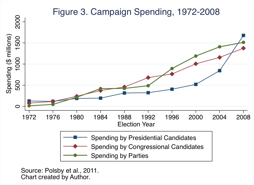
Despite the overwhelming majority of Americans accounting for a decreasing share of total income, as well as stagnating real annual wages,[13] spending on national political campaigns –presidential and congressional – has increased substantially since the 1970s. Figure 3, which shows campaign spending by all presidential and congressional candidates throughout each election cycle from 1972 to 2008, presents this trend graphically. During this period, total campaign spending by presidential candidates increased from roughly $127 million in 1972 to over $1.6 billion in 2008 (a 1,220% increase), with spending nearly doubling (98%) from 2004 to 2008 alone.[14] Similarly, congressional campaign spending increased by roughly 1,600% from $77 million in 1972 to $1.375 billion in 2008.[15] Had these congressional figures simply kept up with inflation, campaign spending would have amounted to only $435 million in 2008 – roughly one third of the actual amount spent.[16] Incredibly, these trends in campaign finance all occurred prior to the Citizens United ruling in 2010, which suggests that this phenomenon is symptomatic of something much deeper than the court decision.
These trends of inequality and campaign spending coincide with another development: the erosion of public financing of campaigns. Prior to 2000, most candidates participated in a federal system of matching funds that limited the amount of campaign spending.[17] In 2000, George W. Bush became the first presidential candidate from a major party to opt out of this system in the nominating process. According to Brendan Doherty, a political scientist at the United States Naval Academy, Bush concluded that it was in his best interest to opt out, which allowed him to raise larger amounts of money with fewer limits on how that money was spent.[18]
For instance, had Bush accepted public matching, he would have been required to limit spending prior to the Republican National Convention to $40.5 million and would have received $16.9 million in matching.[19] By comparison, Bush was able to raise $95 million for the nominating process by opting out of public matching.[20] In 2008, candidates from both major parties opted out of matching funds for both the primary and general elections, thus enabling them to raise far greater amounts of money than would have been possible from public matching. Candidates, acting in their political self-interest, are simply going where the money is.
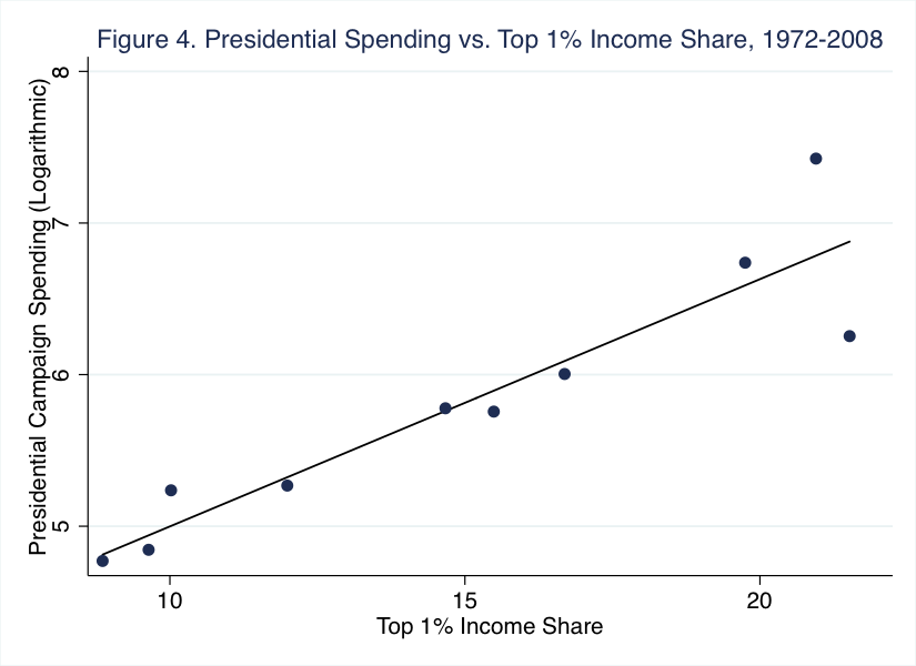
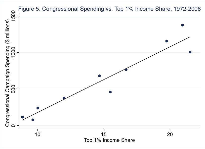
If the vast majority of Americans account for a diminishing share of income, they should – in theory – be spending less and less of their disposable income on campaign donations. However, the amount of money raised and spent on political campaigns has not adhered to this logic, and is instead trending in the opposite direction. These campaign funds must be coming from somewhere, and the evidence suggests that candidates are likely procuring them from those who can most afford it: the wealthiest Americans. Figure 4 correlates the level of campaign spending from each election cycle (1972-2008) with the corresponding income shares for that year.[21] As this figure shows, there exists a strong correlation between the top 1% income share and presidential campaign spending. As Figure 5 further reveals, a nearly identical trend occurs at the congressional level as well. Together, these two correlations suggest a relationship between the income shares of the top 1% and spending on presidential and congressional campaigns.
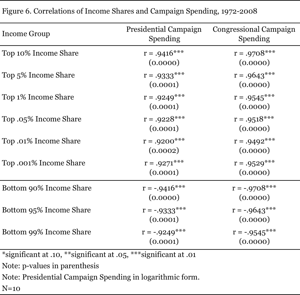
The correlation coefficients – displayed in Figure 6 – of each income group’s share with presidential and congressional campaign spending reveal remarkably consistent results across the board. Each top income group – from the top 10% to top .001% – exhibits a very strong positive correlation with presidential campaign spending. Further, each correlation coefficient is statistically significant at the 99% level, five out of six of which are significant at 99.99%. The inverse of this trend is evident with the bottom 90% to 99% income shares, which reveal negative correlations of similar magnitude. Moreover, these correlations become even stronger when each variable is correlated with congressional campaign spending.
Regression Analysis
With correlation established between income share and the level of campaign spending, a simple regression analysis reveals possible causation between these variables. While a multiple regression – with the inclusion of alternative and control variables – would be ideal for testing multiple variables that may influence the level of campaign spending at the margins, my sample size of ten observations makes such a technique impractical. Hence, this section uses multiple single regressions between each of the independent variables (all representative of top incomes) listed in Figure 6 for both presidential and congressional campaign spending. It is also important to note that due to the small sample size, this analysis treats the data as cross-sectional rather than time series, which means that the errors presented here are likely to be underestimated. Nonetheless, the levels of statistical significance leave me confident that a time-series replication of this model will yield similar results.
The simple linear regression model employed for measuring the effect of top incomes on presidential spending can be written as the log-level regression,
Log(Presidential Spending) = β1(Income Share) + ε,
where presidential spending is represented in its logarithmic form to account for a severe rightward skew of its distribution. Similarly, a comparable linear regression is used for congressional spending:
(Congressional Spending) = β1(Income Share) + ε.
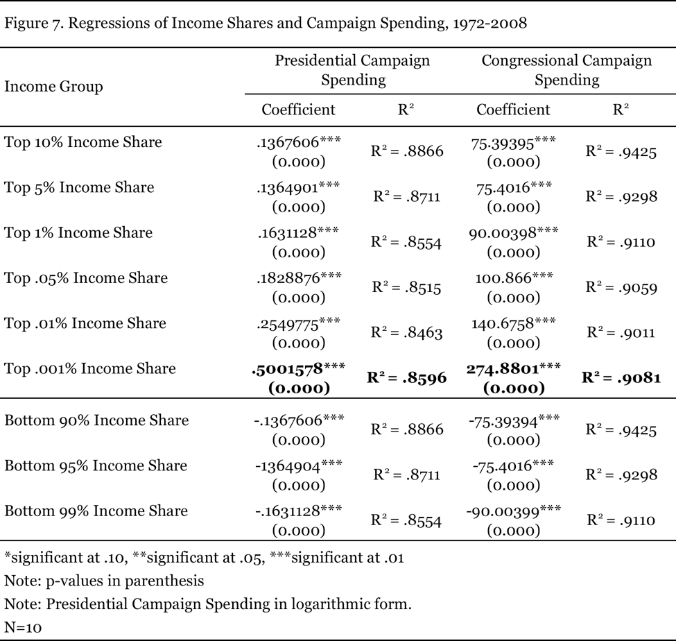
The results of these models are shown in Figure 7, which presents the values of the coefficients, the level of statistical significance, and the r2 values. Evidently, each independent variable fit the data well, with r2 values ranging from .8463 (top .01% income share) to .8866 (top 10% income share). In addition, the coefficients for each measure of top income share are statistically significant at the 99.9% level. Among these results, however, the most salient predictor of presidential campaign spending is the income share of the very richest Americans, the top .001% – the likes of whom are often corporate executives and financiers.[22] As the model suggests, as the income share of this top 1% of the 1% increases by one percentage point, the amount of presidential campaign spending increases by a roughly 50%. This finding supports those found by previous empirical studies, such as the work of Bonica, McCarty, Poole, and Rosenthal, who find that both Democrats and Republicans have relied heavily on donations from the top .01% in recent decades.[23]
Similarly, congressional campaign spending also appears to be highly influenced by income share. Each independent variable fits the data well, with r2 values ranging from .9425 (top 10% income share) to .9011 (top .01% income share). Furthermore, congressional campaign spending shows comparable increases in its coefficients with each step up the income scale, with the top .001% exhibiting the strongest influence. For instance, as the income share of the top .001% increases by an additional percentage point, the level of congressional campaign spending increases by roughly $275 million. These results suggest that while the income shares of the top 10% to 1% of Americans are leading to higher levels of campaign spending, the top .001% – the very richest Americans – is really the driving force behind the increases shown in Figure 3. Intuitively, this implies that as the income distribution becomes even more unequal in coming years, national politics should become even more flush with campaign contributions from the wealthiest Americans.
Evidence from the States
The same analysis can be conducted at the state level to see if states where the top earners account for a larger share of income provide more campaign contributions than less unequal states. To test this, data were collected on state-level income shares of the top 1% by consulting the work of Estelle Sommeiller and Mark Price, researchers at the Economic Policy Center.[24] While Sommeiller and Price’s dataset – which captures the income shares of the top 1% of earners within each state – does not include data for the same years outlined above, it does contain values for 2007, as well as the total change in income share from 1979 to 2007 (by state). From these values, I calculated the average annual top 1% income growth over this 28-year period and estimated figures for 2000, 2004, 2008, and 2012. Consulting the Center for Responsive Politics’ data on campaign contributions, by state, for these four election cycles, the same national analysis conducted above was replicated for each of the four years.[25] Measuring this relationship over these election cycles – before and after the Citizens United decision – allows for both the visualization of the trend over time, as well as the exacerbating effect of the Supreme Court’s ruling.
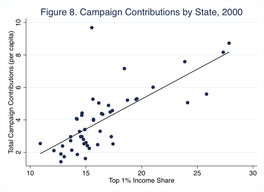
The correlations between top 1% income share by state and campaign contributions are presented in Figures 8 through 11. In each election year, there exists a positive, statistically significant correlation between the share of income that the top 1% accounts for in that state and the amount of per capita campaign contributions made in that state.[26] Evidently, states where the top 1% maintains a greater income share consistently give more campaign contributions, per capita, than states with more equal income distributions. When looking at these correlations in sequential order, notice how the data points move upward and to the right in each new election cycle, which implies that state campaign contributions are growing as the top 1% income share grows. In 2000, for instance, no state gave more than $10 in per capita campaign contributions.[27] By 2008, however, a number of states exceeded this amount and the entire plot simply shifted upward as the axes changed. After Citizens United, the data points all shifted dramatically, as is evident by comparing the y-axes from 2000 to 2012.
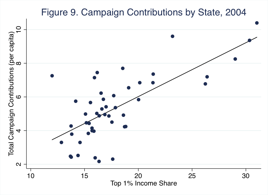
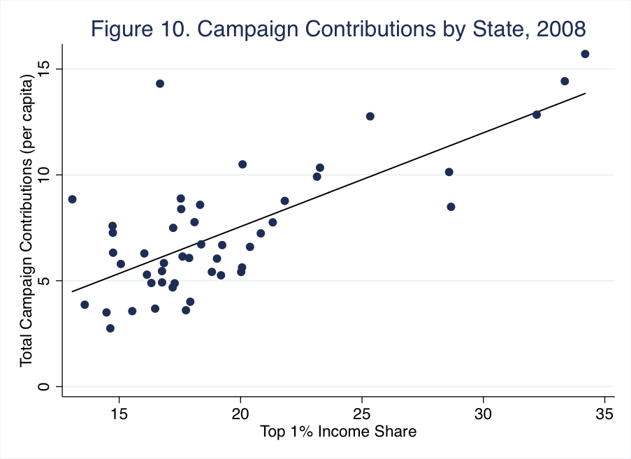
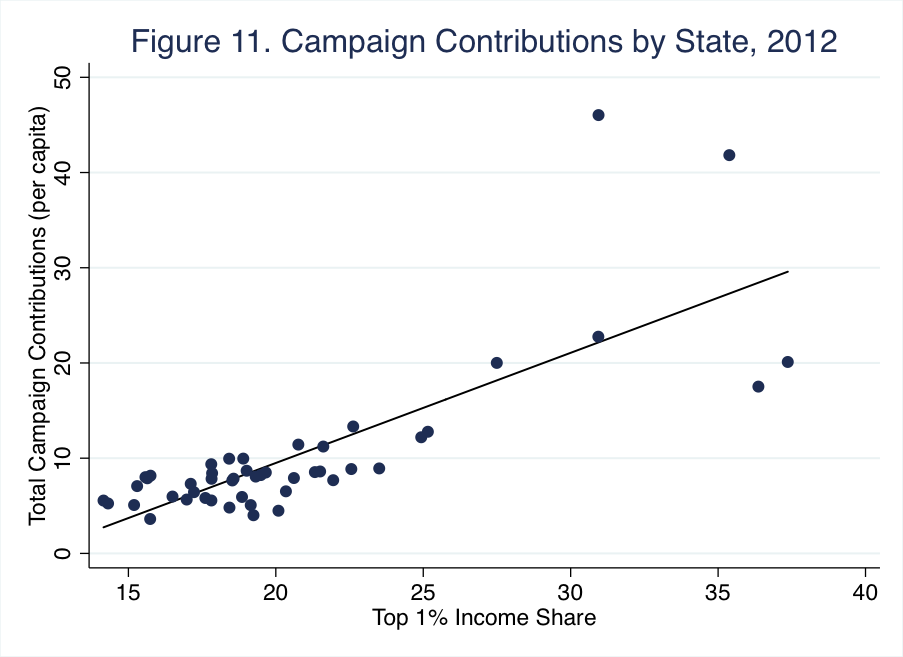
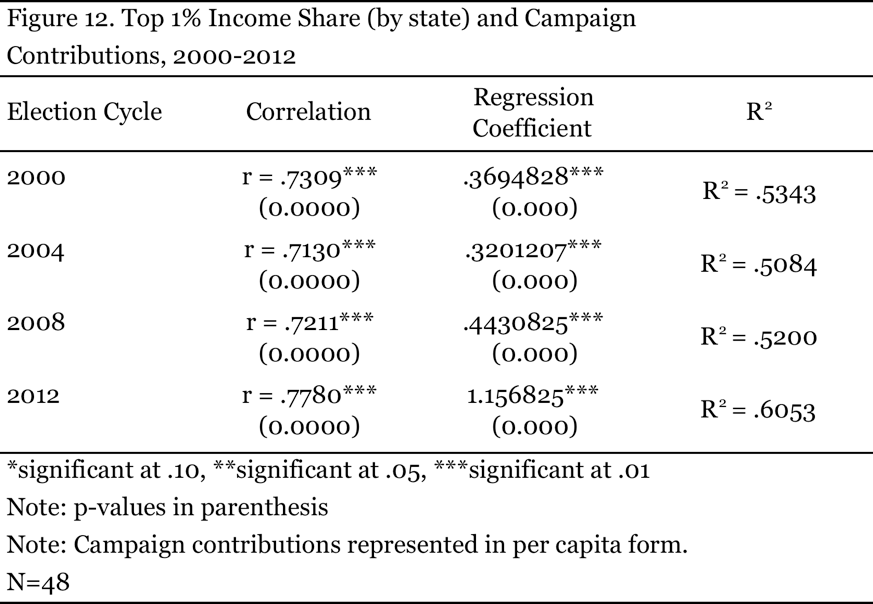
These correlations are all statistically significant at the 99.99% level and are consistent across each election cycle, which suggests that they are not the result of some rare phenomena during a single election. In addition, the correlation coefficients, displayed in Figure 12, are consistent across each election and become stronger as the top 1% garners a larger share of income in each state. To further examine whether this correlation translates into causation, a simple regression model was employed:
(Per Capita Campaign Contributions) = β1(Top 1% Income Share) + ε.
The results of these regressions suggest causation between the top 1% income share in each state and the amount of per capita campaign contributions. Moreover, this trend – despite dipping briefly in the wake of the dot-com collapse – was exacerbated by the 2010 Citizens United decision. For instance, in 2004, each additional percentage point in the top 1% income share was associated with an additional $0.32 in state per capita campaign contributions. By 2008, this effect increased to $0.44 for every percentage point increase, before nearly tripling to $1.15 per percentage point in 2012. Nevertheless, despite this considerable shift after the Supreme Court’s ruling, the trend was evident – albeit not as pronounced – in the election cycles prior to 2012. Overall, this suggests that while Citizens United did cause a significant increase in the level of money in politics, it is more of a culmination of the trend rather than the commencement.
Possible Alternative Arguments
While these results suggest that growing income inequality is responsible for the prevalence of money in politics, there are potential counterarguments to this argument. These alternatives, however, do not sufficiently undermine nor dispute the evidence presented in this article. For instance, the first main counterargument rests on what is arguably the most common explanation for the level of money in politics: Citizens United. While the Citizens United decision did exacerbate the level of money in politics by allowing for both greater sums of money while decreasing the transparency of donations, it is not the root cause. As advanced in this article, the amount of spending by presidential campaigns – funded primarily through donations – has been increasing since the 1970s at remarkable rates. The findings presented here, which show that the income share of the richest Americans is strongly influencing both presidential and congressional campaign spending, are derived from pre-Citizens United election cycles (1972-2008). Over this period, the amount of money in politics increased by over 1,000% at both the presidential and congressional level. If Citizens United were the main cause of this trend, the levels of campaign spending prior to the decision should have exhibited a much flatter trend – or at least one more in-line with inflation.
Another possible counterargument is that the level of money in politics is simply the result of a systemically weak public financing system. As mentioned in this article, this is certainly plausible; the public financing system for elections has become nearly obsolete given the availability of private donations from wealthy donors. This counterargument, however, is largely unconvincing due to the fact that candidates from both major parties utilized the public financing system for over two decades prior to the 2000 election cycle.[28] If the public funding system was systemically inferior for financing campaigns as opposed to private funding, we should have observed a trend of candidates opting out much earlier and with more frequency than what actually occurred.
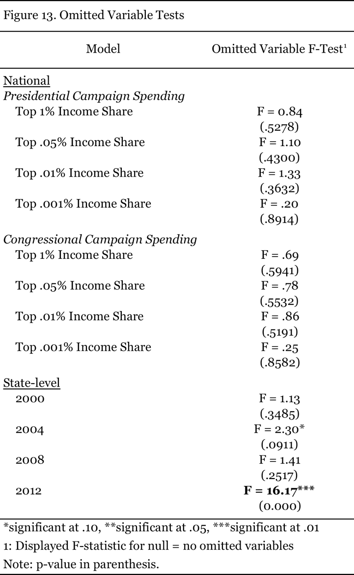
Finally, some may take issue with the methods used in this article and contend that other variables, in addition to income inequality, may be significantly influencing the level of money in politics. Admittedly, while there may be factors around the margins that slightly affect these trends, the majority of the variation can be statistically explained by income share. Figure 13 displays the statistical omitted variable tests for each of the regressions presented above. As expected, all tests for omitted variables return negative, with the exception of 2012, the first election in the wake of Citizens United. Intuitively, this suggests that until the Supreme Court’s momentous decision, the income share of the wealthiest Americans was indeed a sound predictor for explaining most of the variation in campaign contributions and spending.
Policy Implications and Conclusion
The evidence presented in this article suggests that income inequality is responsible for the plethora of money in politics. While Citizens United has certainly played a factor since its ruling in 2010, the top 1% income share – whether at the national or state level – has been one of the strongest predictors of the level of money in politics for years, even decades. Hence, focusing on overturning Citizens United as a policy remedy for the current state of campaign finance in America – as many, particularly on the Democratic side of the aisle, advocate for – is simply incomplete. Certainly, reversing the Citizens United decision would have a significant impact in curtailing the level of money in politics, but it would not reverse the underlying trend of income inequality. Being cognizant of this point may allow for more comprehensive and robust solutions to an issue that has been – quite literally – decades in the making. This section briefly explores a number of policy options that may, in addition to reversing Citizens United, lead to far less money in politics.
Go Where the Money Is: The 1% of the 1%
As Figure 7 suggests, the income share of the top 1% is a salient predictor of the level of money in politics. This influence, however, is far from equal. The income shares of the top 10% to .05% lead to a roughly 13 to 18% increase in the level of presidential campaign spending as these income share increases by one percentage point. Though sizable, particularly when considering that presidential campaigns are already extraordinarily expensive, these amount to pennies in comparison to the influence of the top .01% and top .001%, whose each additional percentage point of income share leads to an increase in presidential campaign spending by 25% and 50%, respectively. Moreover, these individuals also have the most influence on congressional campaign spending, ranging from an additional $140 million to $274 million, respectively, with each additional spending for each percentage point increase in their income shares.
Implementing policies that stand to make the income distribution less uneven may thus have the most substantial impact on decreasing the prevalence of money in politics. As Bakija et al. and Bonica et al. describe, top earners that fall within the upper echelons of the income distribution are not numerous. Nonetheless, simply closing loopholes and implementing stricter donation restrictions would be inadequate for a number of reasons. First, it is highly unlikely that politicians would go against the interests of this powerful constituency – one that they rely on for sizable campaign contributions. Hence, any legislation that seeks to impose restrictions on top earners would be lobbied heavily, and politicians have been shown to listen to affluent constituents.[29] Second, any campaign finance restrictions that do manage to be implemented may not be durable if those at the top continue to garner a larger share. The political influence of those at the top of the income distribution will only continue to grow as their income grows, thus enabling them to influence future politicians to ease restrictions, as has been done in the past. Essentially, restricting spending without addressing the enormous disparities in both income and influence would neither be a sustainable nor lasting solution. Thus, the most viable, durable solution for reducing the amount of money in politics is to address the underlying trend of income inequality. In doing so, the enabling factor through which the wealthiest Americans acquire so much political influence would be far more proportional.
Reform of Public Financing of Campaigns
Regardless of how even the income distribution becomes, it could be that a proverbial “Pandora’s Box” has already been opened in terms of how campaigns are financed. If opting out of public funding, as has been the trend in recent elections, provides candidates with the best chance to win, they are likely to do so regardless of the income distribution. Hence, more can be done to make public financing the more attractive option relative to relying solely on private donations. Thus, another policy option, though only effective in conjunction with reducing income inequality, is to make the public funding of campaigns an attractive option. Presidents, being goal-oriented political actors, often respond to the rules of the game in which they operate.[30] George W. Bush, for example, did not opt out of public financing due to an ideological opposition or because he wished to set a trend of more money in politics. Rather, Bush decided to forego public funds because doing so provided him with a better chance of winning the presidency.[31] If candidates can garner exponentially greater amounts of campaign resources without public funds, no candidate – no matter how much they dislike the amount of money in politics – is going to choose to restrict him or herself. Even President Obama, an opponent of the Citizens United decision, claimed that he would not “unilaterally disarm” while his opponents had millions of dollars pouring in from wealthy donors.[32] To change these incentives, the system would need to be reformed to make public financing more attractive.
Such reform could be done in a number of ways. Restrictions could be placed on the amount of funds a candidate is eligible to raise from private sources so that the difference between public and private financing is not so consequential. This would enable candidates who choose to rely on public matching to remain electorally competitive. Another option would be to impose a strict spending limit that covers both public and private financing. For example, this would mean that despite the amount of money raised by each candidate or the source of those funds (whether from public matching or private donations), they would only be allowed to spend a certain amount of money in each campaign cycle, indexed for inflation. This would effectively cap the amount of money that candidates are able to spend and thus decrease the incentive to raise excessive funds. A third option may be to implement limits on donation size while introducing a tiered system that matches smaller donations at higher rates than larger donations. For example, donations under a certain threshold may be matched 15:1 while donations above a certain amount may not be matched at all. While income may still be distributed unequally, such a system would ensure that influence is not.
Conclusion
As Paul Krugman once asked, “Can anyone seriously deny that our political system is being warped by the influence of big money, and that the warping is getting worse as the wealth of a few grows ever larger?”[33] This article stands to answer this question with the evidence. Although the conventional wisdom in explaining the prevalence of money in politics focuses largely on Citizens United, campaign spending has been increasing for over three decades. Over this same period, the income shares of the top 1% – a symptom of growing inequality – have also increased substantially. As demonstrated in this article, these two phenomena are inextricably linked. For more than three decades, the income share of the richest Americans has exhibited a strong correlation with the level of money in politics. As those at the top of the income distribution account for an increasing share of total income, their ability to spend money on campaign contributions also increases. It may be possible to reverse this trend, however, through greater economic equality and more proportional influence by those at the bottom and middle of the income distribution. While durable solutions can mitigate these trends, effective policy nevertheless requires a cognizance of these underlying trends. For policymakers and advocates to enact the right campaign finance solutions, they should begin by looking where the money is. Hopefully, this article may turn some of their heads in the right direction.
References
Bakija, Jon, Adam Cole, and Bradley T. Heim. (2010). “Jobs and Income Growth of Top Earners and the Causes of Changing Income Inequality: Evidence from U.S. Tax Return Data.” Department of Economics Working Paper 2010-24. Williamstown, MA: Williams College.
Bartels, Larry M. (2005). “Economic Inequality and Political Representation.” Princeton, NJ: Prince Working Group on Inequality.
Bivens, Josh, Gould, Elise, Mishel, Lawrence, Shierholz, Heidi. (2014). “Raising America’s Pay: Why It’s Our Central Economic Policy Challenge,” Economic Policy Institute (Briefing Paper #378).
Bonica, Adam, and Nolan McCarty, Keith T. Poole, and Howard Rosenthal. (2013). “Why Hasn’t Democracy Slowed Rising Inequality?” Journal of Economic Perspectives, 27(3).
Center for Responsive Politics. (2000, 2004, 2008, 2012). “Contributions by State.” Washington, DC: Center for Responsive Politics. Available at: https://www.opensecrets.org/bigpicture/statetotals.php?cycle=2012.
Dahl, Robert A. (1961). Who Governs? Democracy and Power in an American City. New Haven, CT: Yale University Press.
Epstein, Jennifer. (2012). “Obama: `not going to just unilaterally disarm’ on super PACs.” Politico. Available at: http://www.politico.com/news/stories/0212/72882.html.
Krugman, Paul. (2011). “Oligarchy, American Style.” The New York Times. Available at http://www.nytimes.com/2011/11/04/opinion/oligarchy-american-style.html.
Muller, Jerry. (2013). “Capitalism and Inequality: What the Right and the Left Get Wrong.” Foreign Affairs, March/April 2013 Issue.
Polsby, Nelson W., Wildavsky, Aaron B., Schier, Steven E., and Hopkins, David A. (2011). Presidential Elections: Strategies and Structures of American Politics (13th ed.). Lanham, MD: Rowman & Littlefield.
Saez, Emmanuel. (2013). “Striking it Richer: The Evolution of Top Incomes in the United States (Updated with 2012 preliminary estimates).” Pathways Magazine, Palo Alto: Stanford Center for the Study of Poverty and Inequality.
Sommeiller, Estelle, and Mark Price. (2015). “The Increasingly Unequal States of America: Income Inequality by State, 1917-2012.” Washington, DC: Economic Policy Institute.
Stiglitz, Joseph. (2013). The Price of Inequality: How Today’s Divided Society Endangers Our Future. New York, NY: W.W. Norton & Company.
U.S. Census Bureau. (2008). “Table 1: Annual Estimates of the Resident Population for the United States, Regions, States, and Puerto Rico: April 1, 2000 to July 1, 2008.” Washington, DC: U.S. Census Bureau.
Wilkinson, R. & Pickett, K. (2011). The Spirit Level: Why Greater Equality Makes Societies Stronger. New York: Bloomsburg Press.
- Nelson W. Polsby, Aaron B. Wildavsky, Steven E. Schier, and David A. Hopkins, Presidential Elections: Strategies and Structures of American Politics (13th ed.), Lanham, MD: Rowman & Littlefield, 2011, p. 54. ↑
- Emmanuel Saez, “Striking it Richer: The Evolution of Top Incomes in the United States (Updated with 2012 preliminary estimates),” Pathways Magazine, Palo Alto: Stanford Center for the Study of Poverty and Inequality, 2013. ↑
- Nelson W. Polsby et al., Presidential Elections: Strategies and Structures of American Politics (13th ed.). ↑
- Emmanuel Saez, “Striking it Richer: The Evolution of Top Incomes in the United States,” Table A3: Top fractiles income shares (including capital gains) in the United States. ↑
- Ibid. ↑
- Ibid. ↑
- Ibid. ↑
- Richard G. Wilkinson and Kate Pickett, The Spirit Level: Why Greater Equality Makes Societies Stronger, New York: Bloomsburg Press, 2011. ↑
- Robert A. Dahl, Who Governs? Democracy and Power in an American City, New Haven, CT: Yale University Press, 1961, p. 1. ↑
- Larry M. Bartels, “Economic Inequality and Political Representation,” Princeton, NJ: Prince Working Group on Inequality, 2005. ↑
- Ibid. ↑
- Joseph Stiglitz, The Price of Inequality: How Today’s Divided Society Endangers Our Future, New York, NY: W.W. Norton & Company, 2013, p. 120. ↑
- Josh Bivens, Elise Gould, Lawrence Mishel, and Heidi Shierholz, “Raising America’s Pay: Why It’s Our Central Economic Policy Challenge,” Economic Policy Institute (Briefing Paper #378), 2014.From 1979 – 2012, the bottom 90% of earners saw a cumulative real annual wage increase of only 17.1%, compared to 153.6% of the top 1%. ↑
- Nelson W. Polsby et al., Presidential Elections: Strategies and Structures of American Politics (13th ed.). ↑
- Ibid. ↑
- Brendan J. Doherty, The Rise of the President’s Permanent Campaign, Lawrence, Kansas: University Press of Kansas, 2012, p. 28. ↑
- Ibid. ↑
- Ibid. ↑
- Ibid. ↑
- Ibid. ↑
- Data was retrieved from the aforementioned referenced works of Polsby et al. and Saez. ↑
- Jon Bakija, Adam Cole, and Bradley T. Heim, “Jobs and Income Growth of Top Earners and the Causes of Changing Income Inequality: Evidence from U.S. Tax Return Data,” Department of Economics Working Paper 2010-24, Williamstown, MA: Williams College, 2010. ↑
- Adam Bonica, Adam, Nolan McCarty, Keith T. Poole, and Howard Rosenthal, “Why Hasn’t Democracy Slowed Rising Inequality?” Journal of Economic Perspectives, 27(3), 2013. ↑
- Estelle Sommeiller and Mark Price, “The Increasingly Unequal States of America: Income Inequality by State, 1917-2012,” Washington, DC: Economic Policy Institute, 2015. ↑
- Incorporating Census population data and measuring the per capita campaign contributions controls variation in state population. ↑
- These contribution figures include both presidential and congressional elections. ↑
- District of Columbia, Virginia and Maryland are excluded from these correlations and regressions to control for their proximity to Washington, DC. For example, Washington, DC is very unequal (Gini over .5) and donates an incredible amount of donations. In 2008, Washington, DC – home to many important lobbies – averaged $418 in per capita contributions; an obvious outlier. Given the distortion in the figures from the Beltway, Virginia and Maryland were excluded to ensure that this was controlled for. ↑
- Brendan J. Doherty, The Rise of the President’s Permanent Campaign, Lawrence, Kansas: University Press of Kansas, 2012, p. 35. ↑
- Larry M. Bartels, “Economic Inequality and Political Representation,” Princeton, NJ: Prince Working Group on Inequality, 2005. ↑
- Brendan J. Doherty, The Rise of the President’s Permanent Campaign, Lawrence, Kansas: University Press of Kansas, 2012, p. 26. ↑
- Ibid, p. 35. ↑
- Jennifer Epstein, “Obama: `not going to just unilaterally disarm’ on super PACs,” Politico, 2012. ↑
- Paul Krugman, “Oligarchy, American Style,” The New York Times, 2011. ↑